
CAS MONOGRAPH SERIES
NUMBER 4
USING THE ODP BOOTSTRAP MODEL:
A PRACTITIONER’S GUIDE
Mark R. Shapland
CASUALTY ACTUARIAL SOCIETY

ere are many papers that describe the over-dispersed Poisson (ODP) bootstrap
model, but these papers are either limited to the basic calculations of the model or
focus on the theoretical aspects of the model and always implicitly assume that the
ODP bootstrap model is perfectly suited to the data being analyzed. In order to use
the ODP bootstrap model on real data, the analyst must rst test and review the
assumptions of the model and may need to consider various modications to the basic
algorithm in order to put the ODP bootstrap model to practical use. is monograph
starts by gathering the evolutionary changes from dierent papers into a complete ODP
bootstrap modeling framework using a standard notation. en it generalizes the basic
model into a more exible framework. Next it describes the adjustments or enhancements
required for practical use and addresses the diagnostic testing of the model assumptions.
While this monograph is focused on the ODP bootstrap model, we must recognize that
it is a special subset of a larger framework of models and that there are a wide variety of
other stochastic models that should also be considered. However, since no single model
is perfect we also explore ways to combine or credibility weight the ODP bootstrap model
results with various other models in order to arrive at a “best estimate” of the distribution,
similar to how a deterministic best estimate is generally derived in practice. Finally, the
monograph will also extend the model to illustrate the GLM Bootstrap and the model
output to address other risk management issues and suggest areas for future research.
Keywords. Bootstrap, Over-Dispersed Poisson, Reserve Variability, Reserve Range,
Distribution of Possible Outcomes, Generalized Linear Model, Best Estimate.
Availability of
Excel workbooks. In lieu of technical appendices, several
companion Excel workbooks are included that illustrate the calculations described in this
monograph. The companion materials are summarized in the Supplementary
Materials section and are available at https://www.casact.org/sites/default/
files/2021-02/practitionerssuppl-shaplandmonograph04.zip. Other sources of ODP
bootstrap modeling software that could be used for educational purposes would include
working parties and other industry groups in North America and Europe, including
but not limited to models freely available in the R statistical software package.

Casualty Actuarial Society
4350 North Fairfax Drive, Suite 250
Arlington, Virginia 22203
www.casact.org
(703) 276-3100
USING THE ODP BOOTSTRAP MODEL:
A PRACTITIONER’S GUIDE
Mark R. Shapland
Using the ODP Bootstrap Model: A Practitioner’s Guide
By Mark R. Shapland
Copyright 2016 by the Casualty Actuarial Society
All rights reserved. No part of this publication may be reproduced, stored in a retrieval system, or
transmitted, in any form or by any means, electronic, mechanical, photocopying, recording, or otherwise,
without the prior written permission of the publisher. For information on obtaining permission for use of
material in this work, please submit a written request to the Casualty Actuarial Society.
Library of Congress Cataloguing-in-Publication Data
Shapland, Mark R.
Using the ODP Bootstrap Model: A Practitioner’s Guide
ISBN 978-0-9968897-4-2 (print edition)
ISBN 978-0-9968897-5-9 (electronic edition)
1. Actuarial science. 2. Loss reserving. 3. Insurance—Mathematical models.
I. Shapland, Mark
1. Introduction .................................................................................................... 1
1.1. Objectives ................................................................................................2
2. Notation ........................................................................................................... 4
3. e Bootstrap Model ....................................................................................... 6
3.1. Origins of Bootstrapping ..........................................................................7
3.2. e Over-Dispersed Poisson Model ..........................................................8
3.3. Variations on the ODP Model ................................................................14
3.4. e GLM Bootstrap Model ....................................................................16
4. Practical Issues ............................................................................................... 20
4.1. Negative Incremental Values ...................................................................20
4.2. Non-Zero Sum of Residuals ...................................................................23
4.3. Using an N-Year Weighted Average ........................................................23
4.4. Missing Values ........................................................................................24
4.5. Outliers ..................................................................................................24
4.6. Heteroscedasticity ..................................................................................25
4.7. Heteroecthesious Data............................................................................27
4.8. Exposure Adjustment .............................................................................29
4.9. Tail Factors .............................................................................................29
4.10. Fitting a Distribution to ODP Bootstrap Residuals ................................30
5. Diagnostics .................................................................................................... 31
5.1. Residual Graphs .....................................................................................32
5.2. Normality Test .......................................................................................33
5.3. Outliers ..................................................................................................36
5.4. Parameter Adjustment ............................................................................37
5.5. Model Results ........................................................................................41
6. Using Multiple Models .................................................................................. 45
6.1. Additional Useful Output ......................................................................49
6.2. Estimated Cash Flow Results ..................................................................49
6.3. Estimated Ultimate Loss Ratio Results ...................................................50
6.4. Estimated Unpaid Claim Runoff Results ................................................51
6.5. Distribution Graphs ...............................................................................51
6.6. Correlation .............................................................................................53
Contents
iv Casualty Actuarial Society
Contents
7. Model Testing ................................................................................................ 56
7.1. Bootstrap Model Results ........................................................................56
7.2. Future Testing ........................................................................................57
8. Future Research ............................................................................................. 58
9. Conclusions ................................................................................................... 59
APPENDICES ...................................................................................................... 63
Appendix A—Schedule P, Part A Results ..........................................................65
Appendix B—Schedule P, Part B Results ..........................................................78
Appendix C—Schedule P, Part C Results .........................................................91
Appendix D—Aggregate Results ....................................................................104
Appendix E—GLM Bootstrap Results ...........................................................108
References ........................................................................................................... 111
Selected Bibliography ......................................................................................... 114
Abbreviations and Notations .............................................................................. 115
About the Author ................................................................................................ 116
e concept of bootstrapping generally invokes the idea that once a process has been
started, it can replicate without additional external input. Disciplines from biology and
physics to business and statistics use bootstrapping to analyze numerous processes. For
example, in statistics, bootstrapping involves starting with one sample and using it to
derive many more subsamples drawn from the original sample. A specialized applica-
tion within actuarial science involves derivation of a distribution of possible outcomes
for each step in the loss development process.
Considerable literature has been developed over the past twenty-plus years regarding
bootstrapping as it relates to actuarial science and the loss reserving process. In this work,
Mr. Shapland collects the research from this vast literature base and frames it in one
comprehensive presentation. e result is a complete over-dispersed Poisson (ODP)
bootstrap model. At the same time, those who have worked with ODP bootstrapping
know that these models have limitations when using real-world data. Mr. Shapland’s work
also proposes modifications and enhancements that allow more practical application of
the ODP bootstrap model. In addition, he provides details on generalized linear models,
of which the ODP bootstrap is one form.
With the knowledge that model risk is a real risk—no single model is perfect—
Mr. Shapland further explores ways to combine the results of ODP bootstrapping with
other types of models in an effort to determine a true “best estimate” of the distribution.
A set of illustrative Excel files, along with detailed instructions on how to use them,
complements this monograph. With these files, the reader can follow through, step by
step, the theory presented in monograph.
is monograph provides a one-stop shop for practical application of bootstrapping
for the loss reserving process. e Monographs Editorial Board thanks the author for a
valuable contribution to the casualty actuarial literature.
Leslie R. Marlo
Chairperson
Monograph Editorial Board
Foreword
Leslie R. Marlo, Editor in Chief
Emmanuel Bardis
Brendan P. Barrett
Craig C. Davis
Ali Ishaq
C. K. Stan Khury, consultant
Glenn G. Meyers, consultant
Katya Ellen Press, consultant
2016 CAS Monograph Editorial Board
Casualty Actuarial Society 1
e term “bootstrap” has a colorful history that dates back to German folk tales of
the 18th century. It is aptly conveyed in the familiar cliché admonishing laggards to
“pull oneself up by their own bootstraps.” A physical paradox and virtual impossibility,
the idea has nonetheless caught the imagination of scientists in a broad array of elds,
including physics, biology and medical research, computer science, and statistics.
Bradley Efron (1979), Chairman of the Department of Statistics at Stanford Uni-
versity, is most often associated as the source of expanding bootstrapping into the realm
of statistics, with his notion of taking one available sample and using it to arrive at many
others through resampling.
In actuarial science, the concept of bootstrapping has become increasingly common
in the process of loss reserving. e most commonly cited examples are England and
Verrall (1999; 2002), Pinheiro, et al. (2003), and Kirschner, et al. (2008), who combine
the bootstrap concept with a basic chain ladder model. ese papers detail a form of
the model where the incremental losses are modeled as over-dispersed Poisson random
variables. In this monograph, it is called the over-dispersed Poisson bootstrap model, or
the ODP bootstrap. e goal of the ODP bootstrap model is to generate a distribution
of possible outcomes, rather than a point estimate, providing more information about
the potential results.
At the present time, the vast majority of reserving actuaries in the U.S. are focused on
deterministic point estimates. is is not surprising as the American Academy of Actuaries’
primary standard of practice for reserving, ASOP 36, is focused on deterministic
point estimates and the actuarial opinion required by regulators is also focused on
deterministic estimates. However, actuaries are moving towards estimating an unpaid
claim distribution, encouraged by the following factors:
• ASOP 43 denes “actuarial central estimate” in such a way that it could include
either deterministic point estimates or a rst moment estimate from a distribution;
• the SEC is looking for more reserving risk information in the 10-K reports led by
publicly traded companies;
• all of the major rating agencies have built or are building dynamic risk models to
help with their insurance rating process and welcome the input of company actuaries
regarding unpaid claim distributions;
• companies that use dynamic risk models to help their internal risk management
processes need unpaid claim distributions;
1. Introduction
2 Casualty Actuarial Society
Using the ODP Bootstrap Model: A Practitioner’s Guide
• e Solvency II regime in Europe is moving many insurers towards unpaid claim
distributions; and
• International Financial Accounting Standards, while still being discussed, shows
actuaries that the future of insurance accounting may rely on unpaid claim
distributions for booked reserves.
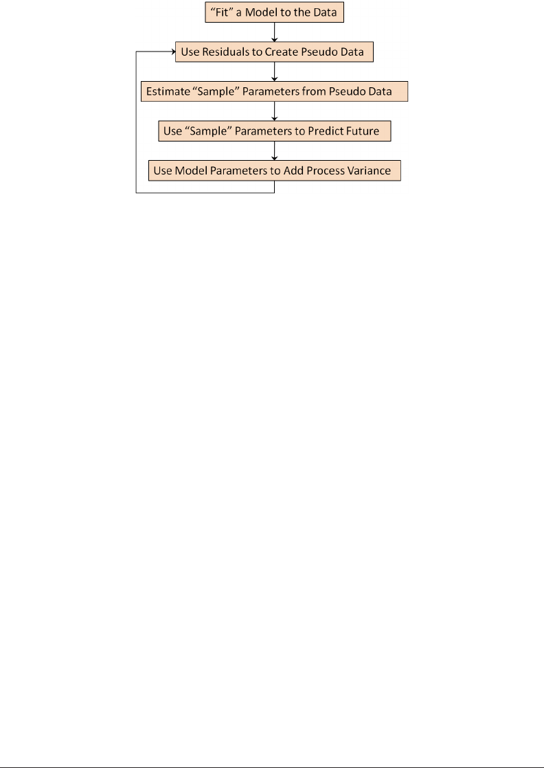
1.1. Objectives
One objective of this monograph is to provide more practical details on the Generalized
Linear Model (GLM), of which the ODP bootstrap model
1
is a specic form. A GLM
allows the user to “t” the model to the data, as illustrated in Figure 1.1. e benet
of a GLM is that it can be specically tailored to the statistical features found in the
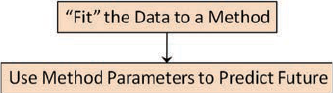
data under analysis. In contrast, consider algorithms that essentially force the data to
be “t” to a static method in order to predict the future as illustrated in Figure 1.2.
2
If a method does not use parameters or assumptions that t the statistical features
of the data then it may not project a reasonable point estimate. Similarly, if model
assumptions and parameters do not t the statistical features found in the data then the
results of a simulation may not be a very good estimate of the distribution of possible
outcomes. us, the modeling framework must be able to adapt to or “t” the model
to the data so this point will be elaborated on in later sections.
Another objective of this monograph is to show how the ODP bootstrap modeling
framework can be used in practice, to help the wider adoption of unpaid claim distribu-
tions. Most of the papers describing stochastic models, including the ODP bootstrap
model, tend to focus primarily on the theoretical aspects of the model while ignoring
the data issues that commonly arise in practice. As a result the models can be quite
elegantly implemented yet suer from practical limitations such as only being useful
1
Some authors dene a model as having a dened structure and error distribution, so under this more restrictive
denition bootstrapping would be considered to be a method or algorithm. However, using a less restrictive
denition of a model as an algorithm that produces a distribution, bootstrapping would be dened as a model.
2
For most deterministic reserving methods diagnostic tools can be used to test assumptions, adjust parameters and
“t” the method to the data, but not all assumptions can be adjusted and blindly applying a method is equivalent
to a static method.
Figure 1.1. Stochastic Model Diagram
Casualty Actuarial Society 3
Using the ODP Bootstrap Model: A Practitioner’s Guide
for complete triangles or only for positive incremental values. us, while keeping as
close to the theoretical foundation as possible, another objective is to illustrate how
practical adjustments can be made to accommodate common data issues and allow the
model to “t” the data. As a practical matter, it is also possible that the model does not
t the data very well, or less well than other models, so the process of diagnosing the
assumptions will inform the actuary’s judgment when considering how much weight,
if any, to give the model in relation to other models.
Another potential roadblock seems to be the notion that actuaries are still searching
for the perfect model to describe “the” distribution of unpaid claims, as if imperfections
in a model remove it from all consideration since it can’t be “the one.” is notion can
also manifest itself when an actuary settles for a model that seems to work the best or is
the easiest to use, or with the idea that each model must be used in its entirety or not at
all. Interestingly, this notion was dispelled long ago with respect to deterministic point
estimates as actuaries commonly use many dierent methods, which range from easy to
complex, and judgmentally weight the results to arrive at their best estimate.
Model risk—the risk that the model you have chosen is not the same as the one that
generates future losses—is very real and weighting or combining multiple estimates is a
very practical way of addressing model risk. us, another objective of this monograph
is to show how stochastic reserving can be similar to deterministic reserving when it
comes to analyzing and using the best parts of multiple models by illustrating how the
results from an ODP bootstrap model can be weighted together with other models.
More importantly, the monograph hopes to illustrate the advantage of using a more
complete set of risk estimation tools (which can include both stochastic models and
deterministic methods) to arrive at an actuarial best estimate of the distribution of
possible outcomes, rather than to focus on deterministic methods to select the “mean”
and then simply “add on” a simple approximation or use only a favorite model to
turn that selected mean into a distribution.
Figure 1.2. Static Method Diagram

4 Casualty Actuarial Society
2. Notation
e papers that describe the basic ODP bootstrap model use dierent notation,
despite sharing common steps. Rather than pick the notation in one of the papers, the
notation from the CAS Working Party on Quantifying Variability in Reserve Estimates
Summary Report (CAS Working Party 2005) will be used since it is intended to serve
as a basis for further research.
Many models visualize loss data as a two-dimensional array, (w, d ) with accident
period or policy period w, and development age d (think w = “when” and d = “delay”).
For this discussion, we assume that the loss information available is an “upper triangular”
subset for rows w = 1, 2, . . . , n and for development ages d = 1, 2, . . . , n - w + 1. e
“diagonal” for which w + d equals the constant, k, represents the loss information for
each accident period w as of accounting period k.
3
For purposes of including tail factors, the development beyond the observed data
for periods d = n + 1, n + 2, . . . , u, where u is the ultimate time period for which any
claim activity occurs—i.e., u is the period in which all claims are nal and paid in full,
must also be considered.
e monograph uses the following notation for certain important loss statistics:
c(w, d ): cumulative loss from accident
4
year w as of age d.
q(w, d ): incremental loss for accident year w from d - 1 to d.
c(w, n) = U(w): total loss from accident year w when claims are at ultimate values at
time n,
5
or
c(w, u) = U(w): total loss from accident year w when claims are at ultimate values at
time u.
R(w): future development after age d for accident year w, i.e., = U(w) -
c(w, d ).
f (d ): factor applied to c(w, d ) to estimate q(w, d + 1) or can be used more
generally to indicate any factor relating to age d.
3
For a more complete explanation of this two-dimensional view of the loss information, see the Foundations of
Casualty Actuarial Science (2001), Chapter 5, particularly pages 210–226.
4
e use of accident year is used for ease of discussion. All of the discussion and formulas that follow could also
apply to underwriting year, policy year, report year, etc. Similarly, year could also be half-year, quarter or month.
5
is would imply that claims reach their ultimate value without any tail factor. is is generalized by changing n
to n + t = u, where t is the number of periods in the tail.

Casualty Actuarial Society 5
Using the ODP Bootstrap Model: A Practitioner’s Guide
F(d ): factor applied to c(w, d ) to estimate c(w, d + 1) or c(w, n) or can be
used more generally to indicate any cumulative factor relating to age d.
G(w): factor relating to accident year w—capitalized to designate ultimate
loss level.
h(k): factor relating to the diagonal k along which w + d is constant.
6
e(w, d ): a random uctuation, or error, which occurs at the w, d cell.
E(x): the expectation of the random variable x.
Var (x): the variance of the random variable x.
x*: a randomly sampled value of the variable x.
What are called factors here could also be summands, but if factors and summands
are both used, some other notation for the additive terms would be needed. e
notation does not distinguish paid vs. incurred, but if this is necessary, capitalized
subscripts P and I could be used.
6
Some authors dene d = 0, 1, . . . , n - 1 which intuitively allows k = w along the diagonals, but in this case the
triangle size is n × n - 1 which is not intuitive. With d = 1, 2, . . . , n dened as in this monograph, the triangle size
n × n is intuitive, but then k = w + 1 along the diagonals is not as intuitive. A way to think about this which helps
tie everything together is to assume the w variables are the beginning of the accident periods and the d variables
are at the end of the development periods. us, if we are using years then cell c(n, 1) represents accident year n
evaluated at 12/31/n, or essentially 1/1/n + 1.

6 Casualty Actuarial Society
3. The Bootstrap Model
Although many variations of a bootstrap model framework are possible, this monograph
will focus on the most common example which reproduces the basic chain ladder
method—the ODP bootstrap model. Let’s briey review the assumptions of the basic
chain ladder method, because these assumptions are important in understanding the
distribution created by the ODP bootstrap model.
Start with a triangle array of cumulative data:
d
1 2 3 . . . n–1 n
w 1 c(1, 1) c(1, 2) c(1, 3) . . .
c(1, n-1)
c(1, n)
2 c(2, 1) c(2, 2) c(2, 3) . . .
c(2, n-1)
3 c(3, 1) c(3, 2) c(3, 3) . . .
. . . . . . . . .
n–1
c(n-1, 1) c(n-1, 2)
n c(n, 1)
A typical deterministic analysis of this data will start with an array of development
ratios or development factors:
()
()
()
=
−
Fwd
cwd
cwd
,
,
,1
.(
3.1)
en two key assumptions are made in order to make a projection of the known
elements to their respective ultimate values. First, it is assumed that each accident year
has the same development factor. Equivalently, for each w = 1, 2, . . . , n:
()()
=
FwdFd,.
Under this rst assumption, one of the more popular estimators for the development
factor is the weighted average:
∑
∑
()
()
()
=
−
=
−+
=
−+
Fd
cwd
cwd
w
nd
w
nd
ˆ
,
,1
.(
3.2)
1
1
1
1

Casualty Actuarial Society 7
Using the ODP Bootstrap Model: A Practitioner’s Guide
Certainly there are other popular estimators in use, but they are beyond our scope at
this stage yet most are still consistent with our rst assumption that each accident year
has the same factor. Projections of the ultimate values, or c
(w, n) for w = 1, 2, . . . , n are
then computed using:
∏
()() ()
==
−+
=+
cwncwd Fi dnw
id
n
ˆ
,,
ˆ
,for all1
.(
3.3)
1
is part of the claim projection algorithm relies explicitly on the second assumption,
namely that each accident year has a parameter representing its relative level. ese level
parameters are the current cumulative values for each accident year, or c(w, n - w + 1).
Of course variations on this second assumption are also common, but the point is that
every model has explicit assumptions that are an integral part of understanding the
quality of that model.
One variation on the second assumption is to assume that the accident years are
completely homogeneous.
7
In this case we would estimate the level parameter of the
accident years using:
∑
()
−+
=
−+
cwd
nd
w
nd
,
1
.(
3.4)
1
1
Complete homogeneity implies that the observations c(1, d ), c(2, d ), . . . ,
c(n - d + 1, d) are generated by the same mechanism. us, the column averages from
(3.4) would replace the last actual values along the diagonal to calculate an estimate
assuming homogeneity of accident years.
Interestingly, the basic chain ladder algorithm treats the processes generating the
observations as NOT homogeneous
8
and eectively that “pooling” of the data does not
provide any increased eciency.
9
In contrast, it could be argued that the Bornhuetter-
Ferguson (1972) and Cape Cod methods are a “blend” of these two extremes as the
homogeneity of the future expected result depends on the consistency of the a priori
loss ratios and decay rate, respectively.
3.1. Origins of Bootstrapping
Possibly the earliest development of a stochastic model for the actuarial array of
cumulative development data is attributed to Kremer (1982) and the earliest discussion
of bootstrapping is in Ashe (1986). e basic model used by Kremer is described by
England and Verrall (1999) and Zehnwirth (1989), so there will be no further elaboration
here. It should be noted, however, that this model can be extended by considering
alternatives which are discussed in Barnett and Zehnwirth (2000) and Zehnwirth
(1994), Renshaw (1989), Christodes (1990), and Verrall (1991; 2004), among others.
7
Homogeneous data can have a dierent meaning in mathematics, but here we are dening it to mean having
consistent or the same underlying exposures.
8
Meaning the underlying exposures are changing over time and thus the current cumulative results (observation)
for each year are more appropriate for projecting an estimate.
9
For a more complete discussion of these assumptions of the basic chain ladder model see Zehnwirth (1989).

8 Casualty Actuarial Society
Using the ODP Bootstrap Model: A Practitioner’s Guide
10
Generalized Linear Modeling can be done with and without link functions and with a variety of error distributions.
We are only describing here the particular GLM model that leads to the replication of the chain ladder results.
For a more complete treatise on Generalized Linear Modeling, see McCullagh and Nelder (1989).
11
Some authors refer to this as the standard deviation of the posterior distribution.
12
While over-dispersed Poisson, or ODP, are commonly used terms for this model, it is certainly possible for the
scale parameter to be less than one and thus “under-dispersed” Poisson would be more technically correct in that
case. Alternatively, the more general term quasi-Poisson could be used. In addition, we note that the z parameter in
equation 3.5, and some later formulas, could be removed for simplicity since the primary focus of this monograph is
the ODP Bootstrap model, but it is included so we do not lose sight of the fact that the ODP Bootstrap model
is a specialized case of a larger family of models.
3.2. The Over-Dispersed Poisson Model
e genesis of this model into an ODP bootstrap framework originated with
Renshaw and Verrall (1994) when they proposed modeling the incremental claims
q(w, d ) directly as the response, with the same linear predictor as Kremer (1982), but
using a generalized linear model (GLM) with a log-link function and an over-dispersed
Poisson (ODP) error distribution.
10
en, England and Verrall (1999) discuss how a
specic form of this model is identical to the volume weighted chain ladder model, and
use bootstrapping (sampling the residuals with replacement) to estimate a distribution
of point estimates
11
instead of simulating from a multivariate normal distribution for a
GLM. More formally, the following formulas are used to parameterize the GLM.
[] [][]
() () ()
==φ=φEqwd mVar qwdEqwdm
wd wd
z
,and ,, (3.5)
,,
[]
=ηm
wd wd
ln (3.6)
,,
η=+α +β == α=β=,where:1,2,...,; 1, 2,...,;and0.(3.7)
, 11
cwnd n
wd wd
In this case the a parameters function as adjustments to the constant, c, level
parameter and the b parameters adjust for the development trends after the rst
development period. e power, z, is used to specify the error distribution with:
z = 0 for Normal,
z = 1 for Poisson,
z = 2 for Gamma, and
z = 3 for inverse Gaussian.
us, the z parameter species not only the mean-variance relationship, but the
whole shape of the distribution, including higher moments. Alternatively, we can
remove the constant, c, which will cause the a parameters to function as individual
level parameters while the b parameters continue to adjust for the development trends
after the rst development period:
η=α+β= =,where:1,2,...,;and2,3,...,. (3.8)
,
wndn
wd wd
Standard statistical software can be used to estimate parameters and goodness of t
measures. e parameter f is a scale parameter that is estimated as part of the tting
procedure while setting the variance proportional to the mean (thus “over-dispersed”
Poisson for z = 1)
12
. For educational purposes, the calculations to solve these equations

Casualty Actuarial Society 9
Using the ODP Bootstrap Model: A Practitioner’s Guide
for a 10 × 10 triangle are included in the “Bootstrap Models.xlsm” le, but here, and
in the “GLM Framework.xlsm” le, the calculations are illustrated for a 3 × 3 triangle
for ease of exposition. Consider the following incremental data triangle:
1 2 3
1 q(1, 1) q(1, 2) q(1, 3)
2 q(2, 1) q(2, 2)
3 q(3, 1)
In order to set up the GLM model to t parameters to the data we need to do a
log-link or transform which results in:
1 2 3
1 ln[q(1, 1)] ln[q(1, 2)] ln[q(1, 3)]
2 ln[q(2, 1)] ln[q(2, 2)]
3 ln[q(3, 1)]
e model, as described in (3.8), is then specied using a system of equations with
vectors of a
w
and b
d
parameters as follows:
[]
[]
[]
[]
[]
[]
()
()
()
()
()
()
=α+α+α+β+β
=α+α+α+β+β
=α+α+α+β+β
=α+α+α+β+β
=α+α+α+β+β
=α+α+α+β+β
q
q
q
q
q
q
ln 1, 11 0000
ln 2,10 1000
ln 3,10 0100
ln 1, 21 0010
ln 2, 20 1010
ln 1, 31 0011
.(
3.9)
12323
12 323
12323
1232 3
12 32 3
12323
Converting this to matrix notation we have:
YXA(3.10)=×
Where:
[]
[]
[]
[]
[]
[]
()
()
()
()
()
()
=
Y
ln 1, 1
ln 2,1
ln 3,1
ln 1, 2
ln 2, 2
ln 1, 3
,(
3.11)
q
q
q
q
q
q

10 Casualty Actuarial Society
Using the ODP Bootstrap Model: A Practitioner’s Guide
X
1 0000
01000
00100
10010
01010
10011
,and (3.12)=
=
α
α
α
β
β
A. (3.13)
1
2
3
2
3
In this form we can use iteratively weighted least squares or maximum likelihood
13
to solve for the parameters in the A vector (3.13) that minimize the squared dierence
between the Y matrix (3.11) and the solution matrix (3.14):
[]
[]
[]
[]
[]
[]
ln
ln
ln
ln
ln
ln
.(
3.14)
1,1
2,1
3,1
1,2
2,2
1,3
m
m
m
m
m
m
After solving the system of equations we will have:
[]
[]
[]
[]
[]
[]
=η =α
=η =α
=η =α
=η =α +β
=η =α +β
=η =α +β +β
ln
ln
ln
ln
ln
ln .(3.15)
1,11,1 1
2,12,1 2
3,13,1 3
1,21,2 12
2,22,2 22
1,31,3 123
m
m
m
m
m
m
is solution can then be shown as a triangle:
1 2 3
1 ln[m
1,1
] ln[m
1,2
] ln[m
1,3
]
2 ln[m
2,1
] ln[m
2,2
]
3 ln[m
3,1
]
13
Other methods, such as orthogonal decomposition or Newton-Raphson, can also be used to solve for the parameters.
Iteratively weighted least squares and maximum likelihood are both illustrated in the companion Excel les.

Casualty Actuarial Society 11
Using the ODP Bootstrap Model: A Practitioner’s Guide
ese results can then be exponentiated to produce the tted, or expected, incremental
results of the GLM model:
1 2 3
1 m
1,1
m
1,2
m
1,3
2 m
2,1
m
2,2
3 m
3,1
is monograph will refer to this as the “GLM framework” and it is illustrated for
a simple 3 × 3 triangle in the “GLM Framework.xlsm” le. While the GLM framework
is used to solve these equations for the tted results, the usefulness of this framework
is that the tted incremental values (with the Poisson error distribution assumption)
will equal the incremental values that can be derived from volume-weighted average
development factors, as shown in the “GLM Framework.xlsm” le.
14
at is, it can be
reproduced by using the last cumulative diagonal, dividing backwards successively by
each volume-weighted average development factor and subtracting to get the tted
incremental results. is monograph will refer to this method as the “simplied GLM”
or “ODP Bootstrap.” is has three very useful consequences.
First, the GLM portion of the algorithm can be replaced with a simpler development
factor algorithm while still being based on the underlying GLM framework. Second,
the use of the development factors serves as a “bridge” to the deterministic framework
and allows the model to be more easily explainable to others. And, third, for the GLM
algorithm the log-link process means that negative incremental values can often cause
the algorithm to not have a solution, whereas using development factors will generally
allow for a solution.
15
With a model tted to the data, the ODP bootstrap process involves sampling
with replacement from the residuals. England and Verrall (1999) note that the
deviance, Pearson, and Anscombe residuals could all be considered for this process,
but the Pearson residuals are the most desirable since they are calculated consistently
with the scale parameter. e unscaled Pearson residuals, r
w,d
, and scale parameter, f,
are calculated as follows:
()
=
−,
.(
3.16)
,
,
,
r
qwdm
m
wd
wd
wd
z
∑
φ=
−
r
Np
wd
.(
3.17)
,
2
14
Using other than the Poisson assumption (i.e., z ≠ 1), the incremental values may be close to the values from
the development factors, but they will not be equal.
15
More specically, individual negative cell values may not be a problem (by using the negative of the log of the
absolute value in 3.14). If the total of all incremental cell values in a development column is negative, then the
GLM algorithm will fail. is situation will not cause a problem tting the model as a link ratio less than one
will be perfectly useful. However, this may still cause other problems, e.g., the “GLM framework” and “simplied
GLM” may not be equivalent, which we will address in Section 4.
12 Casualty Actuarial Society
Using the ODP Bootstrap Model: A Practitioner’s Guide
Where N = the number of observations, or incremental data cells in the triangle,
which is typically equal to n × (n + 1) ÷ 2, and p = the number of parameters, which
is typically equal to 2 × (n - 1).
16
Sampling with replacement from the residuals can
then be used to create new sample triangles of incremental values using formula 3.18.
Sampling with replacement assumes that the residuals are independent and identically
distributed, but it does not require the residuals to be normally distributed. Indeed, this
is often cited as an advantage of the ODP bootstrap model since whatever distributional
form the residuals have will ow through to the simulation process. Some authors have
referred to this as a “semi-parametric” bootstrap model since we are not parameterizing
the residuals.
=× +*( ,) *. (3.18)
,,
qwdr mm
wd
z
wd
e sample triangle of incremental values can then be cumulated, new average
development factors can be calculated for the sample and applied to calculate a point
estimate for this data, resulting in a distribution of point estimates for some large number
of samples. In England and Verrall (1999) this is the end of the process, but at the
end of the appendix they note that you should also adjust the resulting distribution
by the degrees of freedom adjustment factor (3.19) and the Scale Parameter (3.17), to
eectively allow for over-dispersion of the residuals in the sampling process and add
process variance to approximate a distribution of possible outcomes.
=
−
.(
3.19)f
N
Np
DoF
Later, in England and Verrall (2002), the authors note that the Pearson residuals
(3.16) could be multiplied by the degrees of freedom adjustment factor (3.19) to include
the over-dispersion in the residuals. As calculated in (3.20), these adjusted residuals
are referred to as scaled Pearson residuals. ey also expand the simulation process
by adding process variance to the future incremental values from the point estimates.
To add this process variance, they assume that each future incremental value m
w,d
is
the mean and the mean times the scale parameter, fm
w,d
, is the variance of a gamma
distribution.
17
is revised model could now be described as estimating a distribution
of possible outcomes, which incorporates process variance and parameter variance in the
simulation of the historical and future data.
18
16
e number of data cells could be less than n × (n + 1) ÷ 2 and the number of parameters could be less than
2 × (n - 1). For example, if the incremental values are zeros for the last three columns in a triangle then these cells
would not be included in the total for N and there will be three fewer b parameters since none are needed to t
to these zero values as the development process is completed already.
17
e Poisson distribution could be used to remain more consistent with the underlying theory of the GLM
framework, but it is considerably slower to simulate, so gamma is a close substitute that performs much faster in
simulation although it can be more skewed than the Poisson. Indeed, other distributions could be used as well to
better approximate the observed “skewness” of the residuals from the diagnostics.
18
Some authors refer to this as the full predictive distribution of the cash ows.
Casualty Actuarial Society 13
Using the ODP Bootstrap Model: A Practitioner’s Guide
()
=
−
×
,
.(
3.20)
,
,
,
r
qwdm
m
f
wd
S
wd
wd
z
DoF
However, Pinheiro et al. (2001; 2003) noted that the bias correction for the residuals
using the degrees of freedom adjustment factor (3.20) does not create standardized
residuals, which is an important step for making sure that the residuals all have the
same variance. In order to have standardized Pearson residuals, the GLM framework
requires the use of a hat matrix adjustment factor (3.23).
()
=
−
.(
3.21)
1
HXXWXXW
TT
First, the hat matrix (3.21) is calculated using matrix multiplication of the design
matrix (3.12) and the weight matrix (3.22).
=
00000
00000
00 000
00000
0 000 0
0 0000
(3.22)
1,1
2,1
3,1
1,2
2,2
1,3
W
m
m
m
m
m
m
=
−
1
1
.(
3.23)
,
,
f
H
wd
H
ii
e hat matrix adjustment factor (3.23) uses the diagonal of the hat matrix (3.21). In
Pinheiro et al. (2003) the authors note two important points about the ODP bootstrap
process as described by England and Verrall (1999; 2002). First, the sampling of the
residuals should not include any zero-value residuals, which are typically in the corners of
the triangle.
19
e exclusion of the zero-value residuals is accounted for in the hat matrix
adjustment factor (3.23), but another common explanation is that the zero-value cells
will have some variance but we just don’t know what it is yet so we should sample from
the remaining residuals but not the zeros. Second, the hat matrix adjustment factor (3.23)
is a replacement for, and an improvement on, the degrees of freedom factor (3.19).
20
us, the scaled Pearson residuals (3.20) should be replaced by the standardized
Pearson residuals:
()
=
−
×
,
.(
3.24)
,
,
,
,
r
qwdm
m
f
wd
H
wd
wd
z
wd
H
19
Technically, the two “corner” residuals are zero because they each have a parameter that is unique to that incremental
value which causes the tted incremental value to exactly equal the actual incremental value.
20
is second point was not addressed clearly in Pinheiro et al. (2001), but as the authors updated and claried the
monograph in Pinheiro et al. (2003) this issue was more clearly addressed.

14 Casualty Actuarial Society
Using the ODP Bootstrap Model: A Practitioner’s Guide
However, the scale parameter (3.17) is still calculated as before, although the
standardized Pearson residuals could be used to approximate the scale parameter as
follows:
∑
()
φ=
.(
3.25)
,
2
r
N
H
wd
H
At this point we have a complete basic “ODP bootstrap” model, as it is often
referred to. It is also important to note that the two key assumptions mentioned
earlier, each accident year has the same development factor and each accident year has
a parameter representing its relative level, are equally applicable to this model.
In order for the reader to test out the dierent “combinations” of this modeling
process the “Bootstrap Models.xlsm” le includes options to allow these historical
algorithms to be simulated. e purpose for describing this evolution of the ODP
bootstrap model framework is threefold: rst, to allow the interested reader to better
understand the details of the algorithm and how these papers and their authors have
contributed to the evolution of this model framework; second, to illustrate the value of
collaborative research via dierent published papers and the contributions of dierent
authors; and, third, to provide a solid foundation for continuing the evolutionary
process and to discuss practical adjustments.
3.3. Variations on the ODP Model
When estimating insurance risk it is generally considered desirable to focus on the
claim payment stream in order to measure the variability of the actual cash ows that
directly aect the bottom line. Clearly, changes in case reserves and IBNR reserves
will also impact the bottom line, but to a considerable extent the changes in IBNR are
intended to counter the impact of the changes in case reserves. To some degree, then,
the total reserve movements can act to mask the underlying changes due to cash ows.
On the other hand, the case reserves contain valuable information about potential
future payments so we should not ignore them and use only paid data.
3.3.1. Bootstrapping the Incurred Loss Triangle
e ODP bootstrap model can be used to model both paid and incurred loss data.
Using incurred data incorporates case reserves, thus perhaps improving the ultimate
estimates. However, the resulting distribution from using incurred data will be possible
outcomes of the IBNR, not a distribution of the unpaid.
21
ere are two possible
approaches for modeling an unpaid loss distribution using incurred loss data: modeling
incurred data and convert the ultimate values to a payment pattern, or, modeling paid
and case reserves separately.
Using the rst approach, a convenient way of converting the results of an incurred
data model to a payment stream is to run the paid data model in parallel with the
21
Using incurred data will also create issues in weighting the results of dierent models which will be discussed in
Section 6.

Casualty Actuarial Society 15
Using the ODP Bootstrap Model: A Practitioner’s Guide
incurred data model, and use the random payment pattern from each iteration from
the paid data model to convert the ultimate values from each corresponding iteration
from the incurred data to a payment pattern for each iteration (for each accident year
individually). e “Bootstrap Models.xlsm” le illustrates this concept. It is worth
noting, however, that this process allows the “added value” of using the case reserves
to help predict the ultimate results to work its way into the calculations, thus perhaps
improving the ultimate estimates, while still focusing on the payment stream for
measuring risk. In eect, it allows a distribution of IBNR to become a distribution of
IBNR and case reserves. is process could be made more sophisticated by correlating
some part of the paid and incurred models (e.g., the residual sampling and/or process
variance portions), but that is beyond the scope of this monograph.
e second approach could be accomplished by applying the ODP bootstrap to
the Munich chain ladder model. is has the advantage over the rst approach of not
modeling the paid losses twice, and of explicitly measuring and imposing a framework
around the correlation of the paid and outstanding losses. Since it is so well detailed in
Liu and Verrall (2010), it will not be discussed in detail here.
3.3.2. Bootstrapping the Bornhuetter-Ferguson
and Cape Cod models
Another common issue with using the ODP bootstrap model is that the distribution
for the most recent accident years can produce results with more variance than you
would expect when compared to earlier accident years. is is usually because more
development factors are used to extrapolate the sampled values for the most recent
accident years which, when coupled with random samples of incremental values, can
result in more extreme uctuations in point estimates. is is analogous to one of
the weaknesses of the deterministic paid chain ladder method—a low, or high, initial
observation can lead to an abnormally low, or high, projected ultimate, respectively.
To help alleviate this problem, the Bornhuetter-Ferguson (1972) or generalized
Cape Cod (Struzzieri and Hussian 1998) deterministic methods can be worked into
the underlying ODP bootstrap model, and the deterministic assumptions of these
methods can also be converted to stochastic assumptions. For example, instead of
using deterministic a priori loss ratios for the Bornhuetter-Ferguson model, the a priori
loss ratios can be simulated from a distribution. Similarly, the Cape Cod algorithm can
be applied to every ODP bootstrap model iteration to produce a stochastic Cape Cod
projection that reects the unique characteristics of each sample triangle.
22
e “Bootstrap Models.xlsm” le also illustrates these Bornhuetter-Ferguson and
Cape Cod ODP bootstrap models.
23
22
In addition to being consistent between paid and incurred data, to the extent there is commonality with
deterministic methods the assumptions should also be consistent. For example, it would not make sense to use
one set of a priori loss ratio assumptions for a deterministic Bornhuetter-Ferguson method and a dierent set of
mean assumptions for a modied ODP bootstrap model.
23
More complex implementations of these models could include modifying the underlying assumptions of the
GLM framework which would result in a completely dierent set of residuals, but that is beyond the scope of
this monograph.

16 Casualty Actuarial Society
Using the ODP Bootstrap Model: A Practitioner’s Guide
3.4. The GLM Bootstrap Model
Two limitations of the chain-ladder model, and hence the ODP bootstrap of the
chain-ladder model, is that it does not measure or adjust for calendar-year eects, and
it includes a signicant number of parameters and many would argue that it over-ts
the model to the data.
Another approach is to go back to the original GLM framework. Returning to
formulas (3.5) to (3.8), the GLM framework does not require a certain number of
parameters so we are free to specify only as many parameters as we need to get a robust
model, which can address the over-tting issue. Indeed, it is ONLY when we specify
a parameter for EVERY accident year and EVERY development year and specify a
Poisson error distribution that we end up exactly replicating the volume weighted
average development factors that allow us to substitute the deterministic algorithm
instead of solving the GLM t.
us, using the original GLM framework, which this monograph will refer to as
the “GLM Bootstrap” model, we can specify a model with only a few parameters, but
there are two drawbacks to doing so.
24
First, the GLM must be solved for each iteration
of the bootstrap model (which may slow down the simulation process) and, second, the
model is no longer directly explainable to others using development factors.
25
While
the impact of these drawbacks should be considered, the potential benets of using the
GLM bootstrap can be much greater.
First, having fewer parameters will help avoid over-parameterizing the model.
26
For
example, if we use only one accident year parameter then the model specied using a
system of equations is as follows (which is analogous to formula 3.9):
[]
[]
[]
[]
[]
[]
()
()
()
()
()
()
=α+β+β
=α+β+β
=α+β+β
=α+β+β
=α+β+β
=α+β+β
q
q
q
q
q
q
ln 1, 11 00
ln 2,11 00
ln 3,11 00
ln 1, 2110
ln 2, 2110
ln 1, 3111 (3.26)
123
123
123
12 3
12 3
123
In this case we will only have one accident year parameter and n - 1 develop-
ment trend parameters, but it will only be coincidence that we would end up with the
equivalent of average development factors. Interestingly, this model parameterization
moves us away from one of the common basic assumptions (i.e., each accident year has
its own level) and substitutes the assumption that all accident years are homogeneous.
24
Using the GLM framework allows for many other variations in the specication of models and then bootstrapping
as described in more detail in England and Verrall (1999; 2002) and others, but this monograph will focus on
variations consistent with the framework underpinning the ODP bootstrap model.
25
However, age-to-age factors could be calculated for the tted data to compare to the actual age-to-age factors and
used as an aid in explaining the model to others.
26
Over-parameterization will be addressed more completely in Section 5.

Casualty Actuarial Society 17
Using the ODP Bootstrap Model: A Practitioner’s Guide
Another example of using fewer parameters would be to only use one development
year parameter (while continuing to use an accident-year parameter for each year),
which would equate to the system of equations in (3.27).
[]
[]
[]
[]
[]
[]
()
()
()
()
()
()
=α+α+α+β
=α+α+α+β
=α+α+α+β
=α+α+α+β
=α+α+α+β
=α+α+α+β
q
q
q
q
q
q
ln 1, 11 000
ln 2,10 100
ln 3,10 010
ln 1, 21001
ln 2, 20101
ln 1, 31 00
2(
3.27)
1232
12 32
1232
1232
12 32
1232
In this example the model parameterization moves away from the other common
basic assumption (i.e., each accident year has its own level, but the same development
parameter is used for all periods), and again it would be pure coincidence to end up
with the equivalent of average development factors.
27
It is also interesting to note that
for both of these two examples there will be one additional non-zero residual that can
be used in the simulations because in each case one of the incremental values no longer
has a unique parameter—i.e., for (3.26) q(3, 1) is no longer uniquely dened by a
3
,
and for (3.27) q(1, 3) is no longer uniquely dened by b
3
.
Of course we can take this simplication to its logical extreme and use a model
with only one accident year parameter and one development year parameter, which
would result in the system of equations in as shown in (3.28).
[]
[]
[]
[]
[]
[]
()
()
()
()
()
()
=α+β
=α+β
=α+β
=α+β
=α+β
=α+β
q
q
q
q
q
q
ln 1, 11 0
ln 2,11 0
ln 3,11 0
ln 1, 211
ln 2, 211
ln 1, 31
2(
3.28)
12
12
12
12
12
12
In this example the model parameterization moves away from both of the common
basic assumptions (i.e., each accident year has its own level, and the dierent development
parameter is used for all periods), and again it would be pure coincidence to end up
with the equivalent of average development factors. In this most “basic” model it is
interesting to note that both of the “zero residuals” will now be non-zero and can be
used in the simulations because both corners no longer have a unique parameter.
is exibility allows the modeler to use enough parameters to capture the
statistically relevant level and trend changes in the data without forcing a specic
number of parameters.
28
27
While we have only one parameter to describe the development period trends, if we convert these to development
factors there will be a dierent factor for each period.
28
How to determine which parameters are statistically relevant will be discussed in Section 5.

18 Casualty Actuarial Society
Using the ODP Bootstrap Model: A Practitioner’s Guide
e second benet, and depending on the data perhaps the most signicant, is
that this framework aords us the ability to add parameters for calendar-year trends.
Adding diagonal, or calendar year trend, parameters to (3.8) we now have:
η=α+β+γ= =
=
wndn
kn
wd wdk
,where:1,2,...,; 2, 3,...,;
and2,3,...,. (3.29)
,
A complete system of equations for the (3.29) framework would look like the
following:
[]
[]
[]
[]
[]
[]
()
()
()
()
()
()
=α+α+α+β+β+γ+γ
=α+α+α+β+β+γ+γ
=α+α+α+β+β+γ+γ
=α+α+α+β+β+γ+γ
=α+α+α+β+β+γ+γ
=α+α+α+β+β+γ+γ
q
q
q
q
q
q
ln 1, 11 000000
ln 2,10 100010
ln 3,10 010011
ln 1, 21001010
ln 2, 20101011
ln 1, 31 001111 (3.3
0)
1232323
12 32323
1232323
1232 32 3
12 32 323
1232323
However, there is no unique solution for a system with seven parameters and six
equations, so some of these parameters will need to be removed. A logical starting
point would be to start with a “basic” model with one accident year (level) parameter,
one development trend parameter and one calendar trend parameter and then add
or remove parameters as needed.
29
e system of equations for this basic model is as
follows:
[]
[]
[]
[]
[]
[]
()
()
()
()
()
()
=α+β+γ
=α+β+γ
=α+β+γ
=α+β+γ
=α+β+γ
=α+β+γ
q
q
q
q
q
q
ln 1, 11 00
ln 2,1 101
ln 3,11 02
ln 1, 2111
ln 2, 2112
ln 1, 31 22 (3.31)
122
122
12 2
122
12 2
122
A third benet of the GLM bootstrap model is that it can be used to model data
shapes other than triangles. For example, missing incremental data for the rst few
diagonals would mean that the cumulative values could not be calculated and the
remaining values in those rst few rows would not be useful for the ODP bootstrap.
However, since the GLM bootstrap uses the incremental values the entire trapezoid
can be used to t the model parameters.
30
29
A simple algorithm to add and/or remove parameters in a search for the “optimal” set of parameters is included
in the “Bootstrap Models.xlsm” le, but more complex algorithms are outside the scope of this monograph.
We focus on the “mechanical” aspects of searching for the “optimal” set of parameters in Section 5 in order to
enhance the educational benets.
30
is issue will be examined in more detail in Section 4.
Casualty Actuarial Society 19
Using the ODP Bootstrap Model: A Practitioner’s Guide
It should also be noted that the GLM bootstrap model allows the future expected
values to be directly estimated from the parameters of the model for each sample
triangle in the bootstrap simulation process. However, we must solve the GLM within
each iteration for the same parameters as we originally set up for the model rather than
using development factors to project future expected values (which is a way of tting
the model to each sample triangle).
e additional modeling power that this exible GLM bootstrap model adds to
the actuary’s toolkit cannot be overemphasized. Not only does it allow one to move
away from the two basic assumptions of a deterministic chain ladder method, it allows
for the ability to match the model parameters to the statistical features you nd in the
data, rather than “force” the data to t the model, often with far fewer parameters and
to extrapolate those features. For example, modeling with fewer development trend
parameters means that the last parameter can be assumed to continue past the end of
the triangle which will give the modeler a “tail” of the incremental values beyond the
end of the triangle without the need for a specic tail factor.
While the monograph continues to illustrate the GLM bootstrap with a 3 × 3
triangle, also included in the companion Excel les are a set of “GLM Bootstrap
6___.xlsm” les that illustrate the calculations for these dierent models using a 6 ×
6 triangle. Also, the “Bootstrap Models.xlsm” le contains a “GLM bootstrap” model
for a 10 × 10 triangle that can be used to specify any combination of accident year,
development year, and calendar year parameters, including setting parameters to zero.
e GLM bootstrap model is akin to the incremental log model described in Barnett
and Zehnwirth (2000), so we will leave it to the reader to explore this exibility by
using the Excel le.

20 Casualty Actuarial Society
4. Practical Issues
Now that the basic ODP bootstrap model has been expanded in a variety of ways, it
is important to address some of the key assumptions of the ODP model and some
common data issues.
4.1. Negative Incremental Values
As noted in Section 3.2, because of the log-link used in the GLM framework
the incremental values must be greater than zero in order to parameterize a model.
However, a slight modication to the log-link function will help this common
problem become a little less restrictive. If we use (4.1) as the log-link function, then
individual negative values are only an issue if the total of all incremental values in
a development column is negative, as the GLM algorithm will not be able to nd a
solution in that case.
[]
[]
{}
() ()
()
() ()
>
=
−<
ln ,for ,0,
0for ,0,
ln ,for ,0
.(
4.1)
qwdqwd
qwd
absqwd qwd
Using (4.1) in the GLM bootstrap will help in many situations, but it is quite
common for entire development columns of incremental values to be negative, especially
for incurred data. To give the GLM framework the ability to solve for a solution in this
case we need to make another modication to the basic model to include a constant.
Whenever a column or columns of incremental values sum to a negative value, we can
nd the largest negative
31
in the triangle, set y equal to the largest negative and adjust
the log-link function by making all the incremental values positive.
[]
()()
() ()
=−ψ
+
+
,,
ln ,for all, (4.2)
qwdqwd
qwdqwd
Using the adjusted log-link function (4.2) we can solve the GLM using formulas
(3.7), (3.8), or (3.27). en we use (4.3) to adjust the tted incremental values
31
e largest negative value can either be the largest negative among the sums of development columns (in which
case there may still be individual negative values in the adjusted triangle) or the largest negative incremental value
in the triangle.
Casualty Actuarial Society 21
Using the ODP Bootstrap Model: A Practitioner’s Guide
and the constant y is used to reduce each tted incremental value by the largest
negative.
mm
wd wd
=+ψ
+
(4.3)
,,
e combination of formulas (4.2) and (4.3) allow the GLM bootstrap to handle
all negative incremental values, which overcomes a common criticism of the ODP
bootstrap. Incidentally, these formulas can also be used to allow the incremental log
model described by Barnett and Zehnwirth (2000) to handle negative incremental
values. As long as these formulas are used sparingly, the author believes that the resulting
distribution will not be adversely aected.
When using the ODP bootstrap simulation process, the solution to negative incremental
values needs to focus on the residuals and sampled incremental values since a development
factor less than 1.00 will create negative incremental values in the tted values. More
specically, we need to modify formulas (3.16) and (3.18) as follows:
32
r
qwdm
absm
wd
wd
wd
z
{}
()
=
−
,
.(
4.4)
,
,
,
qwdr absm m
wd
z
wd
*, *.
()
,,
(
)
=×
{}
+ 45.
While the tted incremental values and residuals using the development factor
simplication (ODP bootstrap) will generally not match the GLM framework solution
using (4.1) or (4.2) and (4.3) they should be reasonably close. While the purists may
object to these practical solutions, we must keep in mind that every model is an
approximation of reality so our goal is to nd reasonably close models that replicate the
statistical features in the data rather than only restrict ourselves to “pure” models. After
all, the assumptions of the “pure” models are themselves approximations.
4.1.1. Negative Values During Simulation
Even though we have solved problems with negative values when parameterizing
a model, negative values can still aect the process variance in the simulation process.
When each future incremental value (using m
w,d
as the mean and the mean times the
scale parameter, fm
w,d
, as the variance) is sampled from a gamma distribution to add
process variance, the parameters of a gamma distribution must be positive. In this case
we have two options for using the gamma distribution to simulate from a negative
incremental value, m
w,d
.
Gamma absm absm
wd wd
[]
{} {}
−φ
,(
4.6)
,,
Gamma absm absm m
wd wd wd
[]
{} {}
φ+,2 (4.7)
,,,
32
e use of other types of residuals, as noted in Section 3.2, may also help address the issue of negative incremental
values, but their exposition is left to the interested reader.

22 Casualty Actuarial Society
Using the ODP Bootstrap Model: A Practitioner’s Guide
Using formula (4.6) is more intuitive as we are using absolute values to simulate
from a gamma distribution and then changing the sign of the result. However, since
the gamma distribution is skewed to the right, the resulting distribution using (4.6)
will be skewed to the left. Using formula (4.7) is a little less intuitive, but seems more
logical since adding twice the mean, m
w,d
, will result in a distribution with a mean of
m
w,d
while keeping it skewed to the right (since m
w,d
is negative).
Negative incremental values can also cause extreme outcomes. is is most
prevalent when resampled triangles are created with negative incremental losses in the
rst few development periods, causing one column of cumulative values to sum close
to zero and the next column to sum to a much larger number and, consequentially,
produce development factors that are extremely large. is can result in one or more
extreme iterations in a simulation (for example, outcomes that are multiples of 1,000s
of the central estimate). ese extreme outcomes cannot be ignored, even if the high
percentiles are not of interest, because they may signicantly aect the mean of the
distribution.
In these instances, you have several options. You can 1) remove these iterations
from your simulation and replace them with new iterations, 2) recalibrate your model,
or 3) limit incremental values to a minimum of zero (or some other minimum value).
e rst option is to identify the extreme iterations and remove them from your
results. Care must be taken that only truly unreasonable extreme iterations are removed,
so that the resulting distribution does not understate the probability of extreme
outcomes.
e second option is to recalibrate the model to x this issue. First you must
identify the source of the negative incremental losses. e most theoretically sound
method to deal with negative incremental values is to consider the source of these
losses. For example, it may be from the rst row in your triangle, which was the rst year
the product was written, and therefore exhibit sparse data with negative incremental
amounts. One option is to remove this row from the triangle if it is causing extreme
results and does not improve the parameterization of the model. Or, if they are caused
by reinsurance or salvage and subrogation, then you can model the losses gross of
salvage and subrogation, model the salvage and subrogation separately, and combine
the iterations assuming the values are correlated.
e third option is to constrain the model output by limiting incremental losses to a
minimum of zero, where any negative incremental is replaced with a zero incremental.
33
For each of these options, keep in mind that this is a form of diagnosing a model
by reviewing the simulated results and then searching for a practical solution before
abandoning a model altogether. is does not mean that you should never abandon
a model in favor of a practical adjustment. Indeed, the higher the frequency of the
underlying issue (negative incremental values in this case) the more likely that the
model does not really t the data.
33
While zero is a convenient minimum or lower bound, a small positive number could also be used, in which case
any values less than the minimum are changed to the minimum.

Casualty Actuarial Society 23
Using the ODP Bootstrap Model: A Practitioner’s Guide
4.2. Non-Zero Sum of Residuals
e standardized residuals that are calculated in the ODP bootstrap model are
essentially error terms, and should in theory be independent and identically distrib-
uted with a mean of zero. However, the residuals are random observations of the true
residual distribution, so the average of all the residuals is usually non-zero. If signi-
cantly dierent than zero, then the t of the model should be questioned. If the average
of the residuals is close to zero, then the question is whether they should be adjusted so
that their average is zero. For example, if the average of the residuals is positive, then
re-sampling from the residual pool will not only add variability to the resampled incre-
mental losses, but may increase the resampled incremental losses such that the average
of the resampled loss will be greater than the tted loss.
It could be argued that the non-zero average of residuals is a characteristic of the
data set, and therefore should not be removed. For example, standardized residuals
implies a normal distribution with zero mean, but skewness in the residuals does not
necessarily imply an average of zero. However, if a zero residual average is desired, then
one option is the addition of a single constant to all non-zero residuals, such that the
sum of the shifted residuals is zero.
4.3. Using an N-Year Weighted Average
It is quite common for actuaries to use weighted averages that are less than all years
in their chain-ladder and related methods. Similarly, both the ODP bootstrap and the
GLM bootstrap can be adjusted to only consider the data in the most recent diagonals.
For the GLM framework (and the GLM bootstrap model), we can use only the most
recent L + 1 diagonals (since an L-year average uses L + 1 diagonals) to parameterize
the model. e shape of the data to be modeled essentially becomes a trapezoid instead
of a triangle, the excluded diagonals are given zero weight in the model and we have
fewer calendar year trend parameters if we are using formula (3.29). When running
the GLM bootstrap simulations we will only need to sample residuals for the trapezoid
that was used to parameterize the model as that is all that will be needed to estimate
parameters for each iteration.
For the ODP bootstrap model, we can calculate L-year average factors instead of
all-year factors and only have residuals for the most recent L + 1 diagonals. However,
when running the ODP bootstrap simulations we would still need to create a whole
resampled triangle so that we can calculate cumulative values.
34
But, for consistency,
we would want to use L-year average factors for projecting the future expected values
from these resampled triangles.
e calculations for the GLM bootstrap are illustrated in the companion “GLM
Bootstrap 6 with 3yr avg.xlsm” le. Note that because the GLM bootstrap estimates
parameters for the incremental data, the tted values will no longer match the tted
values from the ODP bootstrap using volume-weighted average development factors.
34
e tted values for the “unused” diagonals would be calculated using the L-year average ratios, but the
corresponding residuals for those diagonals are all excluded from the sampling process.
24 Casualty Actuarial Society
Using the ODP Bootstrap Model: A Practitioner’s Guide
Depending on the data, the tted values from the simplied GLM (ODP bootstrap) may
or may not be a reasonable approximation to the GLM framework (GLM bootstrap).
Note that this discussion of using L-year average factors assumes volume weighted
averages to be consistent with the GLM framework. is also assumes that all of the
diagnostic tests will be adjusted to reect the use of the last L + 1 diagonals, although
this is beyond the scope of the monograph. Finally, other types of averages could be
used (i.e., straight average, average excluding high & low, etc.) to be more consistent
with what actuaries might use in a deterministic analysis, but these typically move
further away from the GLM framework and are beyond the scope of this monograph.
4.4. Missing Values
Sometimes the loss triangle will have missing values. For example, values may be
missing from the middle of the triangle, or a triangle may be missing the oldest diago-
nals, if loss data was not kept in the early years of the book of business.
If values are missing, then the following calculations will be aected:
• Loss development factors
• Fitted triangle—if the missing value lies on the most recent diagonal
• Residuals
• Degrees of freedom
ere are several solutions. e missing value may be estimated using the surrounding
values. Or, the loss development factors can be modied to exclude the missing values,
and there will not be a corresponding residual for those missing values. Subsequently,
when triangles are resampled, the simulated incremental corresponding to the
missing value should still be resampled so that the cumulative values in those rows can
be calculated, but they would still be excluded from the projection process (i.e., not
included with the sample age-to-age factors) to reproduce the uncertainty in the original
dataset.
If the missing value lies on the most recent diagonal, the tted triangle cannot
be calculated in the usual way. A solution is to estimate the value, or use the value in
the second most recent diagonal to construct the tted triangle. ese are not strictly
mathematically correct solutions, and judgment will be needed as to their eect on the
resulting distribution. Of course for the GLM bootstrap model, the missing data only
reduces the number of observations used in the model.
4.5. Outliers
ere may be a few extreme or incorrect values in the original triangle dataset that
could be considered outliers. ese may not be representative of the variability of the
dataset in the future and, if so, the modeler may want to remove their impact from
the model.
ere are several solutions. ese values could be removed, and dealt with in the
same manner as missing values. Another alternative is to identify outliers and exclude
them from the average development factors (either the numerator, denominator, or
both) and residual calculations, as when dealing with missing values, but re-sample the

Casualty Actuarial Society 25
Using the ODP Bootstrap Model: A Practitioner’s Guide
corresponding incremental when re-sampling triangles. In this case we have removed
the extreme impact of the incremental cell, but we still want to include a non-extreme
variability, which is dierent from a missing data cell since in that case the additional
uncertainty of that missing data can be included by continuing to exclude that cell in
the projection process.
e calculations for the GLM bootstrap are illustrated in the companion “GLM
Bootstrap 6 with Outlier.xlsm” le. Again the GLM bootstrap tted values will no
longer exactly match the tted values from the ODP Bootstrap using volume weighted
average development factors, but they should normally be close.
If there are a signicant number of outliers, then this could be an indication that
the model is not a good t to the data. With the GLM bootstrap, new parameters
could be chosen, or the distribution of the error term can be changed (i.e., change the
z parameter). Under the ODP bootstrap model, an L-year weighted average could be
used, instead of an all year weighted average, which may provide a better t to the data,
or, heteroscedasticity may exist. Remember, though, that for the ODP bootstrap model
there is no distribution assumption for the residuals so a signicant number of residual
outliers could just mean that the residuals are quite skewed. One of the nice features
of the ODP bootstrap is that the skewness in the residuals will be reected in the
simulation process which will result in a skewed distribution of possible outcomes.
35
us, removing any outliers (i.e., giving them zero weight) should be done with caution
and would most commonly be done only after understanding the underlying data.
4.6. Heteroscedasticity
As noted earlier, the ODP bootstrap model is based on the assumption that
the standardized Pearson residuals are independent and identically distributed. It is
this assumption that allows the model to take a residual from one development
period/accident period and apply it to the tted loss in any other development period/
accident period, to produce the sampled values. In statistical terms this is referred to
as homoscedasticity (the residuals have the same variance) and it is important that
this assumption is validated.
A common problem is when some development periods have residuals that appear
to be more variable than others—i.e., they appear to have dierent variances. is is
referred to as heteroscedasticity. With heteroscedasticity, it is no longer possible to take
a residual from one development/accident period and deem it suitable to be applied to
any other development/accident period. In making this assessment, you must account
for the credibility of the observed dierences in variance, and also to note that there
are fewer residuals as the development years become older, so comparing development
years is dicult, particularly near the tail-end of the triangle.
36
35
Other methods of handling outliers could also be introduced, e.g., tempering residuals that are further away from
the interquartile range, but the key to any approach is to understand what the residuals represent so an explicit
assumption can be made and the “best” solution can be used.
36
Section 5 will illustrate how to use residual graphs and other statistical tests to evaluate heteroscedasticity.
26 Casualty Actuarial Society
Using the ODP Bootstrap Model: A Practitioner’s Guide
e existence of heteroscedasticity may suggest that the model is not a good t for
the data. Under an ODP bootstrap, there are a number of ad-hoc adjustments that can
be made to address heteroscedasticity, but they may or may not improve the t of the
model to the data. ey also often result in even more parameters in a model which
could already be over-parameterized. In contrast, under a GLM bootstrap the exibility
of choosing the number of parameters to use, the ability to account for any calendar year
trends, and the exibility to choose the distribution of the error term mean that there are
many ways within the model framework itself to improve the t to the data. erefore,
this exibility could remove the heteroscedasticity problem or at least reduce it.
Nevertheless, if the ODP bootstrap model is still to be used, then to adjust for
heteroscedasticity in your data there are at least three options, 1) stratied sampling,
2) calculating hetero-adjustment (or variance) parameters, or 3) calculate non-constant
scale parameters. Stratied sampling is accomplished by grouping those development
periods with homogeneous variances and then sampling only from the residuals in
each group. While this process is straightforward, some groups may only have a few
residuals in them, which limits the amount of variability in the possible outcomes
compared to the other two options and at least partially defeats the benets of random
sampling with replacement.
e second option is to group those development periods with homogeneous
variances and calculate the standard deviation of the residuals in each of the groups.
en calculate h
i
, which is the “hetero-adjustment” factor, for each group, i:
∪
∪
()
()
=≤≤,for each
1(
4.8)
1,
,
h
stdevr
stdevr
ij
i
j
wd
H
iwd
H
All residuals in group i are multiplied by h
i
.
()
=
−
××
,
(4.9)
,
,
,
,
r
qwdm
m
fh
wd
iH
wd
wd
wd
Hi
Now all groups have the same standard deviation and we can sample with replacement
from among all r
iH
w,d
. e original distribution of residuals has been altered, but this can
be remedied. When the adjusted residuals are resampled, the residual is divided by the
hetero-adjustment factor, h
i
, that applies to the development year of the incremental
loss, as shown in (4.10).
=× +(, )
*
.(
4.10)
*
,,
qwd
r
h
mm
i
i
wd wd
By doing this, the heteroscedastic variances we observed in the data are replicated
when the sample triangles are created, but we are able to freely resample with replacement
from the entire pool of heteroscedasticity adjusted residuals. Also note that these factors
are new parameters so it will aect the degrees of freedom, which impacts the scale
Casualty Actuarial Society 27
Using the ODP Bootstrap Model: A Practitioner’s Guide
parameter (3.17) and the degrees of freedom adjustment factor (3.19).
37
Finally, the
hetero-adjustment factors should also be used to adjust the variance by development
period when simulating the future process variance.
e third option is to modify the formula for the scale parameter (3.17) so that
we have a dierent scale parameter for each hetero group, as illustrated in (4.11) and
(4.12).
38
In (4.12) n
i
is the number of residuals in each hetero group.
∑∑
∑
()
φ=
−
=
−
×=
×
−
r
Np
N
Np
r
N
r
N
wd wd
N
Np
wd
(4.11)
,
2
,
2
,
2
∑
()
φ=
×
−
=
r
n
i
N
Np
wd
i
n
i
i
(4.12)
,
1
2
For this option, the dierent scale parameters also amount to new parameters so
the degrees of freedom adjustment factor would likewise be impacted. In this case,
the scale parameters adjust the future process variance, but we also need to calculate
parameters to adjust the residuals as shown in (4.13). ese hetero-adjustment factors,
h
i
, can also be used to adjust the residuals in (4.9) and used in calculating the resampled
loss in (4.10), similar to the second option.
h
i
i
=
φ
φ
(4.13)
While the hetero-adjustment factors in (4.13) are a bit more theoretically sound,
in practice the factors in (4.8) are likely to be very close so the dierences are not likely
to have much impact. Both of these options are illustrated in the “Bootstrap Models.
xlsm” le.
Of course no matter which formula is used, care needs to be exercised as hetero
groups are used toward the tail of the triangle where fewer and fewer observations
stretch the credibility of the resulting factors.
39
Finally, while use of the GLM bootstrap
should reduce the need for hetero factors, the same three options could also be used
for that model too.
4.7. Heteroecthesious Data
e basic ODP bootstrap model requires both a symmetrical shape (e.g., annual
by annual, quarterly by quarterly, etc. triangles) and homoecthesious data (i.e., similar
37
Some authors have suggested adding a factor for each development period to insure homoscedasticity. However,
this adds many more parameters to a model that can already suer from the criticism of over-parameterization.
us, a balance between the need for hetero parameters and parsimony is appropriate. is will be discussed in
more detail in Section 5.
38
For a more detailed development of this third option see England and Verrall (2006). In particular, see Appen-
dixA.1 on pages 266–268.
39
In the discussion of diagnostics in Section 5 it will be noted that the use of the AIC and BIC statistics will
eectively reect the credibility of the development periods.

28 Casualty Actuarial Society
Using the ODP Bootstrap Model: A Practitioner’s Guide
exposures).
40
As discussed above, using an L-year weighted average in the ODP
bootstrap model or adjusting to a trapezoid shape allow us to “relax” the requirement
of a symmetrical shape. Other non-symmetrical shapes (e.g., annual × quarterly data)
can also be modeled with either the ODP bootstrap or GLM bootstrap, but they will
not be discussed in detail in this monograph.
Most often, the actuary will encounter heteroecthesious data (i.e., incomplete
or uneven exposures) at interim evaluation dates, with the two most common data
triangles being either a partial rst development period or a partial last calendar period.
For example, with annual data evaluated as of June 30, partial rst development period
data would have all development periods ending at 6, 18, 30, etc. months, while
partial last calendar period data would have development periods as of 12, 24, 36, etc.
months for all of the data in the triangle except the last diagonal, which would have
development periods as of 6, 18, 30, etc. months. In either case, not all of the data in
the triangle has full annual exposures—i.e., it is heteroecthesious data.
4.7.1. Partial First Development Period Data
For partial rst development period data, the rst development column has a dif-
ferent exposure period than the rest of the columns (e.g., in the earlier example the rst
column has six months of development exposure while the rest have 12). In a determin-
istic analysis this is not a problem as the development factors will reect the change in
exposure. For parameterizing an ODP bootstrap model, it also turns out to be a moot
issue, since the Pearson residuals use the square root of the tted value to make them all
“exposure independent.”
e only adjustment for this type of heteroecthesious data is the projection of
future incremental values. In a deterministic analysis, the most recent accident year
needs to be adjusted to remove exposures beyond the evaluation date. For example,
continuing the previous example the development periods at 18 months and later are
all for an entire year of exposure whereas the six month column is only for six months
of exposure. us, the 6–18 month development factor will eectively extrapolate the
rst six months of exposure in the latest accident year to a full accident year’s exposure.
Accordingly, it is common practice to reduce the projected future payments by half to
remove the exposure from June 30 to December 31.
41
e simulation process for the ODP bootstrap model can be adjusted similarly to
the way a deterministic analysis would be adjusted. After the development factors from
each sample triangle are used to project the future incremental values the last accident
year’s values can be reduced (in the previous example by 50%) to remove the future
exposure and then process variance can be simulated as before. Alternatively, the future
incremental values can be reduced after the process variance step.
40
To the author’s knowledge, the terms homoecthesious and heteroecthesious are new. ey are a combination of
the Greek homos (or ÓμÓς) meaning the same or hetero (or ε
´
τερο) meaning dierent and the Greek ekthesë (or
ε
´
κθεση) meaning exposure.
41
Reduction by half is actually an approximation since we would also want to account for the dierences in
development between the rst and second half years.

Casualty Actuarial Society 29
Using the ODP Bootstrap Model: A Practitioner’s Guide
4.7.2. Partial Last Calendar Period Data
For partial last calendar period data, most of the data in the triangle has annual
exposures and annual development periods, except for the last diagonal which, con-
tinuing our example, only has a 6-month development period. For a deterministic
analysis, it is common to exclude the last diagonal when calculating average develop-
ment factors, then interpolate those factors to project the future values. Similarly to the
adjustments for partial rst development period data, we can adjust the calculations
and steps in the ODP bootstrap model. Instead of ignoring the last diagonal during the
parameterization of the model, an alternative is to adjust or annualize the exposures in
the last diagonal to make them consistent with the rest of the triangle. e tted tri-
angle can be calculated from this annualized triangle to obtain residuals.
During the ODP bootstrap simulation process, development factors can be
calculated from the fully annualized sample triangles and interpolated. en, the last
diagonal from the sample triangle can be adjusted to de-annualize the incremental
values in the last diagonal—i.e., reversing the annualization of the original last diagonal.
e new cumulative values can be multiplied by the interpolated development factors
to project future values. Again, the future incremental values for the last accident year
must be reduced (in the previous example by 50%) to remove the future exposure.
42
4.8. Exposure Adjustment
Another common issue in real data is exposures that have changed dramatically
over the years. For example, in a line of business that has experienced rapid growth or
is being run o. If the earned exposures exist for this data, then a useful option for the
ODP bootstrap model is to divide all of the claim data by the exposures for each
accident year—i.e., eectively using pure premium development instead of total loss
development. is may improve the t of the model to the data.
During the ODP bootstrap simulation process, all of the calculations would be
done using the exposure-adjusted data and only after the process variance step has been
completed would you multiply the results by the exposures by year to restate them in
terms of total values again.
When adjusting the GLM bootstrap for exposure, the model is tted to exposure
adjusted losses, similar to the ODP bootstrap model using exposure. However, under
the GLM, the t to the exposure adjusted losses are also exposure-weighted. at is,
exposure adjusted losses with higher exposure are assumed to have lower variance. For
more details, see Anderson et al. (2007).
For the GLM bootstrap, exposure adjustment could allow fewer accident year
parameter(s) to be used.
4.9. Tail Factors
One of the most common data issues is that claim development is not complete within
the loss triangle and tail factors are commonly used to extrapolate beyond the end of
42
ese heteroecthesious data issues are not illustrated in the “Bootstrap Models.xlsm” le.
30 Casualty Actuarial Society
Using the ODP Bootstrap Model: A Practitioner’s Guide
the data triangle. ere are many common methods for calculating tail factors and a
useful reference in this regard is the CAS Tail Factor Working Party Report (2013). Tail
factors can be added to the ODP bootstrap algorithm and converted from deterministic
to stochastic by assuming that the tail factor parameter follows a distribution. Once
this is added, other considerations such as process variance, hetero-adjustment factors,
etc. can all be extended to include the tail factors.
A key ingredient for all of these considerations is to verify that the simulations in
the tail are reasonable. For example, the tail factor itself represents the accumulation of
incremental factors (i.e., an age-to-ultimate factor) and using just a single factor may
not produce appropriate incremental results so the “extrapolation” of “incremental tail
factors” may be more appropriate. In the “Bootstrap Models.xlsm” le, the tail factors
can be extrapolated for up to 5 years so that one possibility for how these concepts can
be implemented is included in the companion les.
A rough rule of thumb for the tail factor standard deviation is 50% or less of
the tail factor minus one (assuming the tail factor is greater than one). However, this
should be compared to the standard deviations of the age-to-age factors leading up to
the tail in both the actual data triangle and in the simulated results.
As noted at the end of Section 3.4, for the GLM bootstrap model the last development
parameter can continue to apply past the end of the data triangle until the trend results
in no further claim activity, thus indirectly creating a tail factor. In addition to the last
development parameter, the last calendar period parameter would also extend past the
end of the tail until the combination of the two trends resulted in no further claim
activity.
4.10. Fitting a Distribution to ODP Bootstrap Residuals
Because the number of data points used to parameterize the ODP bootstrap model
are limited (in the case of a 10 × 10 triangle to 55 data points or 53 residuals), it is hard
to determine whether the most extreme observation is a one-in-100 or a one-in-1,000
event (or simply, in this example, a one-in-53 event). Of course, the nature of the
extreme observations in the data will also aect the level of extreme simulations in the
results. Judgment is involved here, but the modeler will either need to be satised with
the level of extreme simulations in the results or modify the ODP bootstrap algorithm.
One way to overcome a lack of extreme residuals for the ODP bootstrap model
would be to t a distribution to the residuals and sample from the distribution instead of
from the residuals themselves (e.g., use a normal distribution if the residuals are found
to be normally distributed). is option is beyond the scope of the companion Excel
les, but this could be referred to as parametric bootstrapping of the ODP bootstrap
model. Note however, that as there are a wide variety of other types of models that can
be bootstrapped, either with or without residuals, parametric bootstrapping can be
done in other ways.

Casualty Actuarial Society 31
5. Diagnostics
e quality of any model depends on the quality of the underlying assumptions. When
a model fails to “t” the data, it cannot produce a good estimate of the distribution of
possible outcomes.
43
However, a balance must be considered for parsimony of parameters
and the goodness-of-t. Over-parameterization may cause the model to be less predictive
of future losses. On the other hand, no model will perfectly “t” the data, so the best
you can hope for with any model is that it reasonably represents the data and your
understanding of the processes that impact the data. erefore, diagnostically evaluating
the assumptions underlying a model is important for evaluating whether it will produce
reasonable results or not and whether it should stay in your selected group of reasonable
models which could receive some weight.
e CAS Working Party, in the third section of their report on quantifying variability
in reserve estimates (2005), identied 20 criteria or diagnostic tools for gauging the
quality of a stochastic model. e Working Party also noted that, in trying to determine
the optimal t of a model, or indeed an optimal model, no single diagnostic tool or
group of tools can be considered denitive. Depending on the statistical features found
in the data, a variety of diagnostic tools are necessary to best judge the quality of the
model assumptions and to adjust the parameters of the model. is monograph will
discuss some of these tools in detail as they relate to the ODP bootstrap and the GLM
bootstrap models.
e key diagnostic tests are designed for three purposes: to test various assumptions
in the model, to gauge the quality of the model t to the data, and/or to help guide
the adjustment of model parameters. Some tests are relative in nature, enabling results
from one set of model parameters to be compared to those of another, for a specic
model, allowing a modeler to improve the t of the model. For the most part, however,
the tests can’t be used to compare dierent models. e objective, consistent with the
goals of a deterministic analysis, is not to nd the one best model, but rather a set of
reasonable models.
Some diagnostic measures include statistical tests, providing a pass/fail determination
for some aspects of the model assumptions. is can be useful even though a “fail” does
not necessarily invalidate an entire model; it only points to areas where improvements can
be made to the model or its parameterization. e goal is to nd the sets of models
43
While the examples are dierent, signicant portions of Sections 5 and 6 are based on Milliman (2014) and IAA
(2010).
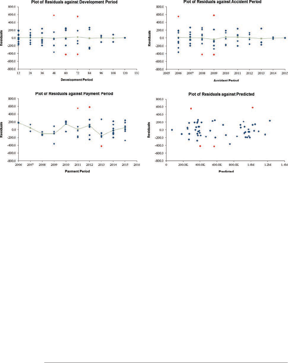
32 Casualty Actuarial Society
Using the ODP Bootstrap Model: A Practitioner’s Guide
and parameters that will yield the most realistic, most consistent simulations, based on
statistical features found in the data.
To illustrate some of the diagnostic tests for the ODP bootstrap model we will consider
data from England and Verrall (1999).
44
5.1. Residual Graphs
e ODP bootstrap model does not require a specic type of distribution for the
residuals, but they are assumed to be independent and identically distributed. Because
residuals will be sampled with replacement during the simulations, this requirement is
important and thus it is necessary to test this assumption. Graphing residuals is a good
way to do this.
Going clock-wise, and starting from the lower-left-hand corner, the graphs in
Figure5.1 show the residuals (blue and red dots
45
) by calendar period, development
period, and accident period and against the tted incremental loss (in the lower-right-
hand corner). In addition, the graphs include a trend line (in green) that highlights the
averages for each period.
At rst glance, the residuals in the graphs appear reasonably random, indicating
the model is likely a good t of the data. But a closer look may also reveal potential
features in the data that may indicate ways to improve the model t.
44
e data triangle was originally used by Taylor and Ashe (1983) and has been used by other authors. is data is
included in the “Bootstrap Models.xlsm” le.
45
In the graphs that follow, the red dots are outliers as identied in Figure 5.7.
Figure 5.1. Residual Graphs Prior to Heteroscedasticity Adjustment
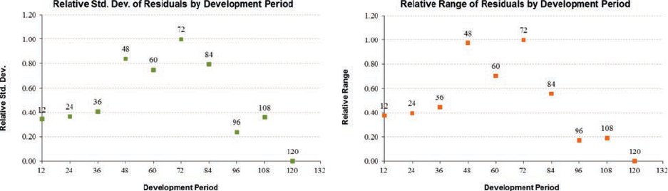
Casualty Actuarial Society 33
Using the ODP Bootstrap Model: A Practitioner’s Guide
e graphs in Figure 5.1 do not appear to indicate issues with un-modeled trends
by accident period or development period (that is, the green “average” lines appear at
at zero). at’s because the ODP bootstrap species a parameter for every accident and
development period. e development-period graph does, however, reveal a potential
heteroscedasticity issue associated with the data—i.e., dierent variances. Note how
the upper left graph appears to show a variance of the residuals in the rst three periods
that diers from those of the middle four or last two periods.
Adjustments for heteroscedasticity can be made with the “Bootstrap Models.xlsm”
le, which enables us to recognize groups of development periods and then adjust the
residuals to a common standard deviation value, as described in Section 4.6. As an aid
to visualizing how to group the development periods into “hetero” groups, graphs of
the standard deviation and range relativities can be developed. Figure 5.2 represents
pre-adjusted relativities for the residuals shown in Figure 5.1 (i.e., prior to adjustment
for factors calculated using either formulas 4.8 or 4.13 and 4.9).
e relativities illustrated in Figure 5.2 help to clarify the changing variability.
However, further testing will be required to assess the optimal groups, which can be
performed using the other diagnostic tests noted below.
e residual plots in Figure 5.3 originate from the same data model after adjusting
for heteroscedasticity using the third option described in Section 4.6 (i.e., using
formulas 4.13 and 4.9). e “hetero” groups chosen are for the rst three, middle four,
and last two development periods, respectively. Determining whether this adjustment
has improved the model will require review of other diagnostic tests.
Comparing the residual plots in Figures 5.1 and 5.3 shows that the residuals now
appear to exhibit the same standard deviation, or homoscedasticity. More consistent rela-
tivities may also be seen in a comparison of the residual relativities in Figures 5.2 and 5.4.
5.2. Normality Test
e ODP bootstrap model does not depend on the residuals being normally
distributed, but even so, comparing residuals against a normal distribution remains
a useful test, enabling comparison of parameter sets and gauging skewness of the
residuals. is test uses both graphs and calculated test values. Figure 5.5 is based on
the data used earlier, before and after the adjustment for heteroscedasticity.
Figure 5.2. Residual Relativities Prior to Heteroscedasticity Adjustment
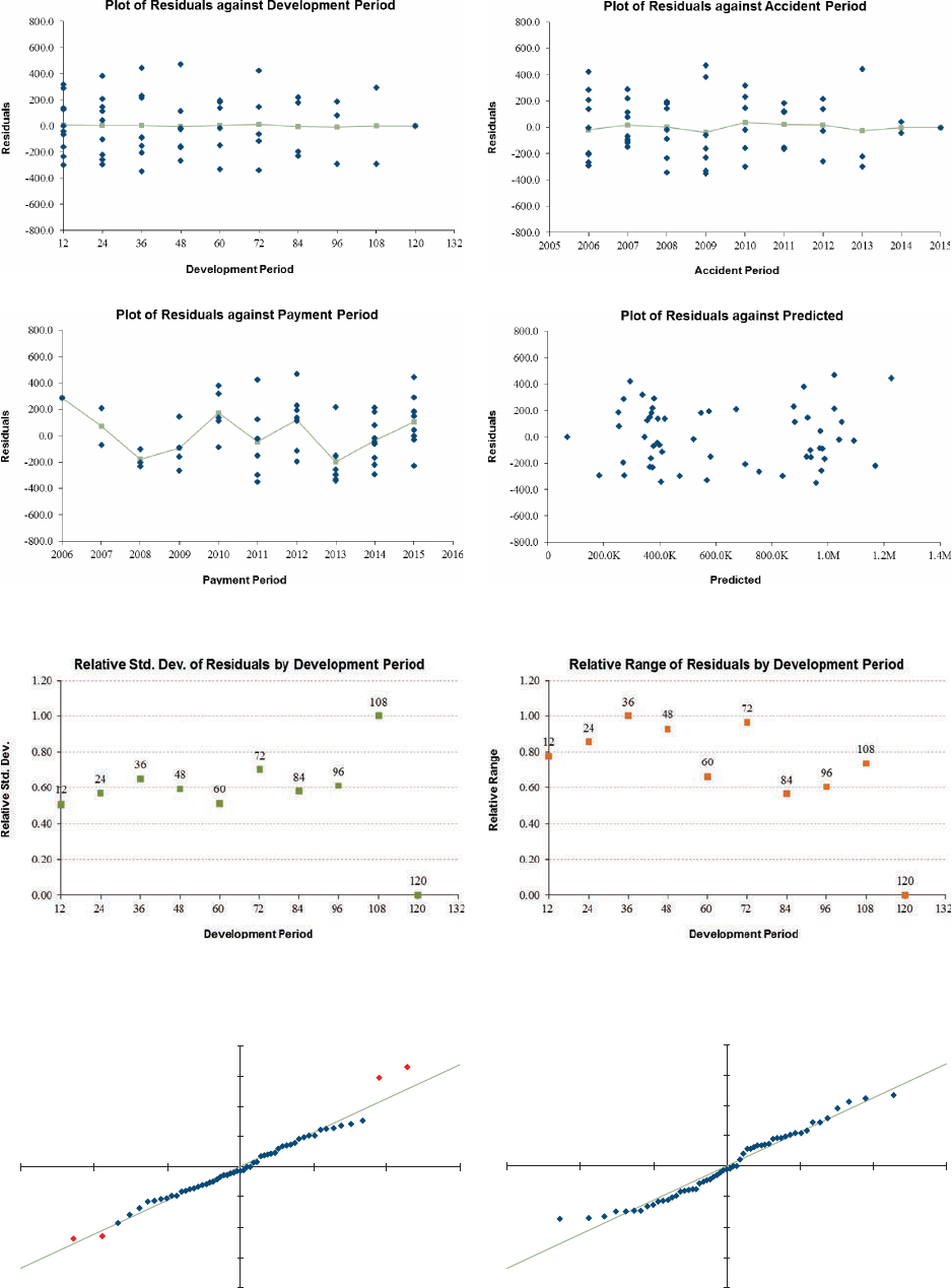
34 Casualty Actuarial Society
Figure 5.3. Residual Graphs After Heteroscedasticity Adjustment
Figure 5.4. Residual Relativities After Heteroscedasticity Adjustment
Figure 5.5. Normality Plots Prior to and After Heteroscedasticity Adjustment
N =55 P-Value = 19.1%R
2
=N =55P-Value = 14.6
%R
2
=
Normal: MU = 1.11, Sigma = 224.08 AIC = 592.2, BIC = 474.2Normal: MU = 1.43, Sigma = 224.07 AIC = 601.3, BIC = 487.3
96.9%97.2%
-800.0
-600.0
-400.0
-200.0
0.0
200.0
400.0
600.0
800.0
-3 -2 -1 0123
Resi duals
Normal Inverse
Normality Plot (Prior to Hetero)
-800.0
-600.0
-400.0
-200.0
0.0
200.0
400.0
600.0
800.0
-3 -2 -1
0123
Resi duals
Normal Inverse
Normality Plot (After Hetero)

Casualty Actuarial Society 35
Using the ODP Bootstrap Model: A Practitioner’s Guide
Even before the heteroscedasticity adjustment, the residual plots appear close to
normally distributed, with the data points tightly distributed around the diagonal
line. e P-value, a statistical pass-fail test for normality, came in at 19.1%, which
exceeds the value generally considered a “passing” score of the normality test, which is
greater than 5.0%.
46
e graphs in Figure 5.5 also show N (the number of data points)
and the R
2
test. After the hetero adjustment, the P-value and R
2
get slightly worse,
which indicates that the heteroscedasticity adjustment has not improved the results
of the diagnostic tests.
While the P-value and R
2
tests assess the goodness of t of the model to the data,
they do not penalize for added parameters. Adding more parameters will almost always
improve the t of the model to the data, but the goal is to have a good t with as few
parameters as possible. Two other tests, the Akaike Information Criteria (AIC) and
the Bayesian Information Criteria (BIC), address this limitation, using the dierence
between each residual and its normal counterpart from the normality plot to calculate
the Residual Sum Squared (RSS) and include a penalty for additional parameters, as
shown in (5.1) and (5.2), respectively.
47
AIC
RSS
.=×+×
××
+
2
2
15
1pn
n
ln
()
π
BIC
RSS
.=×
+×
(
)
n
n
pnln ln
()
52
A smaller value for the AIC and BIC tests indicate residuals that t a normal
distribution more closely, and this improvement in t overcomes the penalty of adding
a parameter.
In our example, with some trial and error, a better “hetero” grouping was found with
the diagnostic results shown in Figure 5.6.
48
For the new “hetero” groups, all of the
statistical tests improved signicantly.
While it might be tempting to add a hetero group for each development column to
improve normality, in general normality can be improved with far fewer groups which
also helps keep the model from being over-parameterized. As an example, if we use
9 hetero groups for the Taylor and Ashe (1983) data the P-value is 14.3%, which is
worse than no groups and only slightly better than the original 3 groups, but the AIC
and BIC increase signicantly.
46
Remember that this doesn’t indicate whether the ODP bootstrap model itself passes or fails—the ODP bootstrap
model doesn’t require the residuals to be normally distributed. While not included in the “Bootstrap Models.
xlsm” le, as discussed in Section 4.10 it could be used to determine whether to switch to a parametric bootstrap
process using a normal distribution.
47
ere are dierent versions of the AIC and BIC formula from various authors and sources, but the general idea
of each version is consistent. Other similar formulas could also be used.
48
In the “Bootstrap Models.xlsm” le the Taylor & Ashe data was entered as both paid and incurred. e rst set
of “hetero” groups are illustrated for the “paid” data and the second set of “hetero” groups are illustrated for the
“incurred” data. e “best” groups were found using the optimization tool shown in the “Groups” sheet.
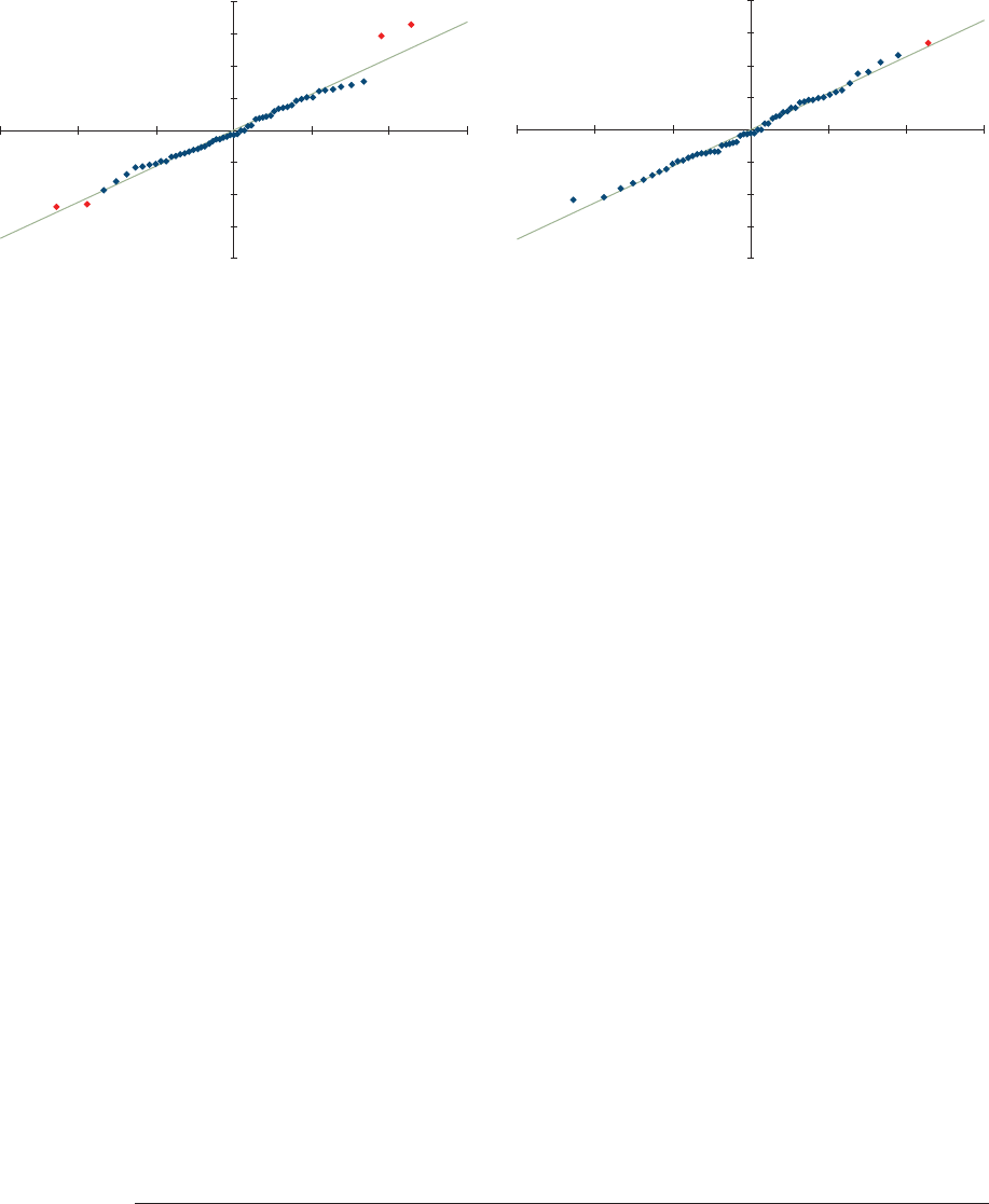
36 Casualty Actuarial Society
Using the ODP Bootstrap Model: A Practitioner’s Guide
5.3. Outliers
Identifying outliers in the data provides another useful test in determining model
t. Outliers can be represented graphically in a box-whisker plot, which shows the
inter-quartile range (the 25th to 75th percentiles) and the median (50th percentile)
of the residuals—the so-called box. e whiskers then extend to the largest values
within three times this inter-quartile range.
49
Values beyond the whiskers may generally
be considered outliers and are identied individually with a point.
Figure 5.7 shows an example of the residuals for the second set of “hetero” groups
(Figure 5.6). A pre-hetero adjustment plot returns four outliers (red dots) in the data
model, corresponding to the two highest and two lowest values in the previous graphs
in Figures 5.1, 5.3, 5.5, and 5.6.
Even after the hetero adjustment, the residuals still appear to contain one outlier.
Now comes a very delicate and often tricky matter of actuarial judgment. If the data
in those cells genuinely represent events that cannot be expected to happen again,
the outlier(s) may be removed from the model (by giving it/them zero weight). But
extreme caution should be taken even when the removal of outliers seems warranted.
e possibility always remains that apparent outliers may actually represent realistic
extreme values, which, of course, are critically important to include as part of any sound
analysis.
Additionally, when residuals are not normally distributed a signicant number of
outliers tend to result, which may only be an artifact of the distributional shape of the
residuals. In this case it is preferable to let these stand in order to enable the simulation
process to replicate this shape. Finally, a signicant number of residuals can also mean
the underlying model is not a good t to the data so other models should be used (see
Section 4.5 for a discussion) or this model given less weight (see Section 6).
49
Various authors and textbooks use widths for the whiskers which tend to span from 1.5 to 3 times the inter-
quartile range. Changing the multiplier will therefore make the box-whisker plot more or less sensitive to
outliers. It is also possible to illustrate “mild” outliers with a multiplier of 1.5 and the more “extreme” outliers
with a multiplier of 3 using dierent colors and/or symbols in the graphs. Of course the actual multipliers can be
adjusted based on personal preference.
Figure 5.6. Normality Plots Prior to and After Heteroscedasticity Adjustment
N =55P-Value = 19.1% R
2
=N =55 P-Value = 89.2
%R
2
=
Normal: MU = 1.11, Sigma = 224.08 AIC = 592.2, BIC = 474.2Normal: MU = 1.28, Sigma = 224.08 AIC = 537.9, BIC = 426.0
99.1%97.2%
-800.0
-600.0
-400.0
-200.0
0.0
200.0
400.0
600.0
800.0
-3 -2 -1 0123
Resi duals
Normal Inverse
Normality Plot (Prior to Hetero)
-800.0
-600.0
-400.0
-200.0
0.0
200.0
400.0
600.0
800.0
-3 -2 -1
0123
Resi duals
Normal Inverse
Normality Plot (After Hetero)
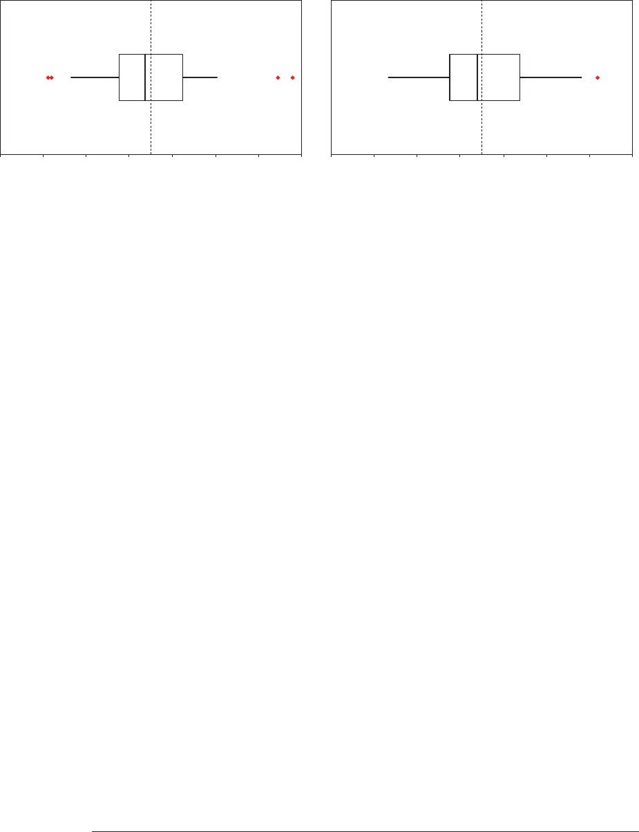
Casualty Actuarial Society 37
Using the ODP Bootstrap Model: A Practitioner’s Guide
While the three diagnostic tests shown above demonstrate techniques commonly
used with most types of models, they are not the only tests available.
50
Next, we’ll take
a look at the exibility of the GLM bootstrap and some of the diagnostic elements of
the simulation results. For a more extensive list of other tests available, see the report,
CAS Working Party on Quantifying Variability in Reserve Estimates (2005).
5.4. Parameter Adjustment
As noted in Section 5.1 the relatively straight average lines in the development and
accident period graphs are a reection of having a parameter for every accident and
development period. In most instances, this is also a strong indication that the model
may be over-parameterized. Using the “GLM Bootstrap” model in the “Bootstrap
Models.xlsm” le we can illustrate the power of removing some of the parameters.
Starting with a “basic” model which includes only one parameter for accident,
development and calendar periods (i.e., only one a, b and g parameter), and adding
vertical brown bars to signify a parameter and vertical red lines to signify no parameter
(i.e., parameter of zero), the residual graphs for the “GLM Bootstrap” model are shown
in Figure 5.8.
e brown bars in the basic model residual graphs represent the parameters and
statistics shown in Table 5.1.
Now for this “basic” model the green average lines show trends in the underlying
data that are not yet captured by the model as well as a parameter for calendar year trend
that is not signicant. For example, the overall development period trend parameter
is -11%, but the underlying data shows a positive trend for the rst 2 or 3 periods
followed by a stronger negative trend for the remaining development periods. Another
way to see that this basic model does not yet provide a good t to the underlying data
is to compare the implied development pattern with that of the ODP bootstrap model,
as shown in Figure 5.9.
50
For example, see Venter (1998).
Interquartile Range = [-147.44, 147.04] Median = Interquartile Range = [-150.62, 175.14
]M
edian =
Outliers = 4 Outliers = 1
-22.04-26.64
-700 -5 00 -300 -100 100300 500700
Box-Whisker Plot (Prior to Hetero)
-700 -5 00 -300 -100 100300 50
0700
Box-Whisker Plot (After Hetero)
Figure 5.7. Box-Whisker Plots Prior to and After Heteroscedasticity Adjustment
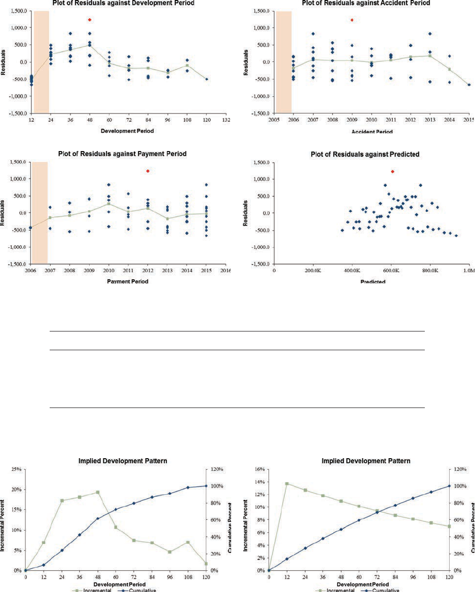
38 Casualty Actuarial Society
Using the ODP Bootstrap Model: A Practitioner’s Guide
Figure 5.8. Residual Graphs for “Basic” GLM Bootstrap Model
Table 5.1. Parameters and Statistics for “Basic” GLM Bootstrap Model
Parm Value Exp(Value) t-Stat Periods
a
1
13.44 686,938 73.92 Accident Years 2006–2015
b
1
(0.11) (3.19) Development Periods 12–132
g
1
0.03 1.08 Calendar Years 2006–2015
ODP Bootstrap Model “Basic” GLM Bootstrap Model
Figure 5.9. Implied Development Patterns
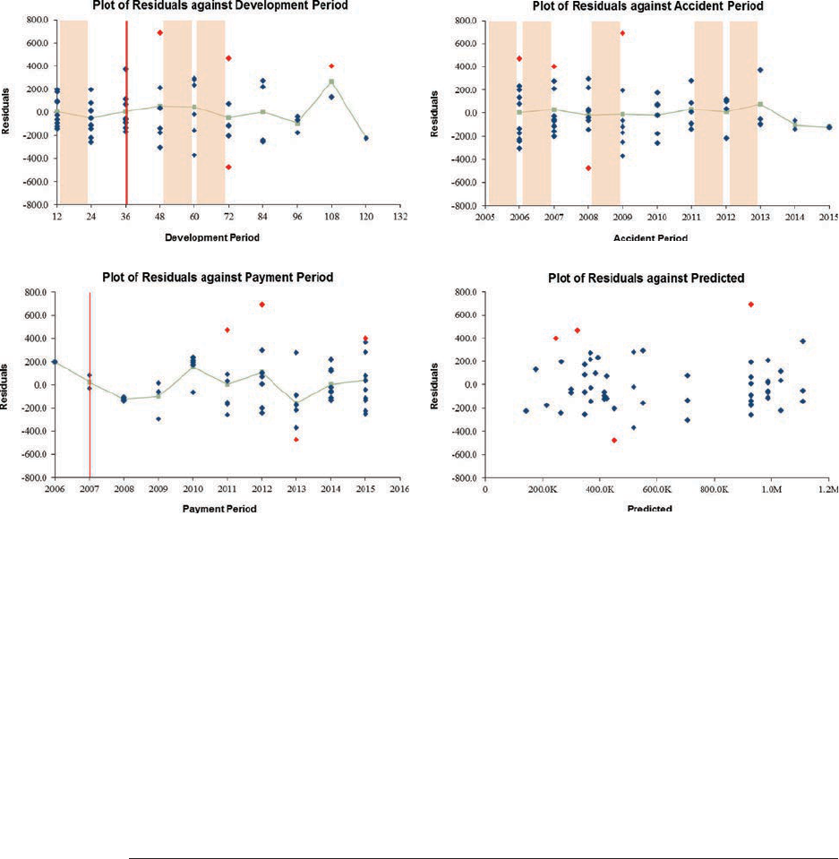
Casualty Actuarial Society 39
Using the ODP Bootstrap Model: A Practitioner’s Guide
With a little trial and error we can nd a reasonably good t to the data using only
ve accident, three development and no calendar parameters as shown in Figure 5.10.
51
In addition to checking the remaining trends in the data with the green average
lines, t-statistics for each new parameter can be checked to make sure each parameter
is statistically signicant.
52
e nal parameters and statistics for the GLM Bootstrap
model are shown in Table 5.2.
Using the “optimal” set of “hetero” groups we can also check the normality graphs
and statistics in Figure 5.11 and outliers in Figure 5.12.
53
Comparing the statistics to the
ODP bootstrap values shown in Figures 5.6 and 5.7, most values improved while some
did not, yet the GLM Bootstrap model is far more parsimonious.
51
In the “Bootstrap Models.xlsm” le the optimization tool in the “GLM” sheet can be used to help nd a good t
for the parameters of the GLM bootstrap. e algorithm for this tool starts with the ODP bootstrap parameters
and then removes the least signicant parameters until only signicant parameters remain. en, if there are
few enough Alpha and Beta parameters, the Gamma parameters are added and removed if not signicant. e
tool does not test to see if a parameter should be zero, so some improvements can sometimes occur by forcing
parameters to equal zero (e.g., compare the parameters from Figure 5.10 to the parameters in the optimization
tool). Finally, it is possible to have a better model t (i.e., lower AIC and/or BIC) with more parameters
even though some of the parameters may not be signicant, so judgment is still appropriate for selection of
parameters.
52
e t-statistic indicates that a parameter is statistically signicant if the absolute value is greater than 2.
53
When using the GLM bootstrap, any selected outliers and hetero groups used for the ODP bootstrap should be
reset and then re-evaluated as they will likely be dierent for the GLM bootstrap. For the “after hetero” portions
of Figures 5.11 and 5.12 the optimization tool in the “Groups” sheet was used.
Figure 5.10. Residual Graphs for GLM Bootstrap Model
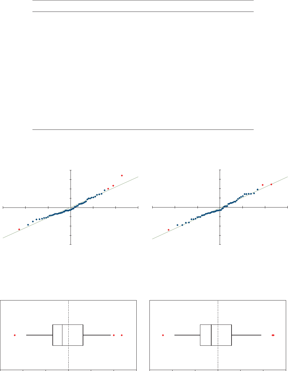
40 Casualty Actuarial Society
Using the ODP Bootstrap Model: A Practitioner’s Guide
Table 5.2. Parameters and Statistics for GLM Bootstrap Model
Parm Value Exp(Value) t-Stat Periods
a
1
12.48 264,036 79.26 Accident Year 2006
a
2
12.82 368,718 2.48 Accident Years 2007–2008
a
3
12.76 347,009 2.11 Accident Years 2009–2011
a
4
12.86 385,644 2.35 Accident Year 2012
a
5
12.93 414,414 3.29 Accident Years 2013–2015
b
1
0.98 7.88 Development Periods 12–24
— 0.00 Development Periods 24–48
b
2
(0.58) (4.88) Development Periods 48–60
b
3
(0.20) (3.29) Development Periods 60–132
— 0.00 Calendar Year 2006–2015
N =55 P-Value = 10.0%R
2
=N =55 P-Value = 64.5
%R
2
=
Normal: MU = 0.68, Sigma = 219.32AIC = 579.5, BIC = 439.5Normal: MU = -12.61, Sigma = 218.95AIC = 535.9, BIC = 399.9
98.5%96.5%
-800.0
-600.0
-400.0
-200.0
0.0
200.0
400.0
600.0
800.0
-3 -2 -1 0123
Resi duals
Normal Inverse
Normality Plot (Prior to Hetero)
-800.0
-600.0
-400.0
-200.0
0.0
200.0
400.0
600.0
800.0
-3 -2 -1
0123
Resi duals
Normal Inverse
Normality Plot (After Hetero)
Figure 5.11. Normality Plots for GLM Bootstrap Model
Interquartile Range = [-138.48, 129.11]Median = Interquartile Range = [-156.62, 119.43
]M
edian =
Outliers = 4 Outliers = 3
-59.65-53.17
-6
00 -400 -200 0 200 400600
Box-Whisker Plot (Prior to Hetero)
-600 -400 -200 0200 40
0600
Box-Whisker Plot (After Hetero)
Figure 5.12. Box-Whisker Plots for “GLM Bootstrap” Model
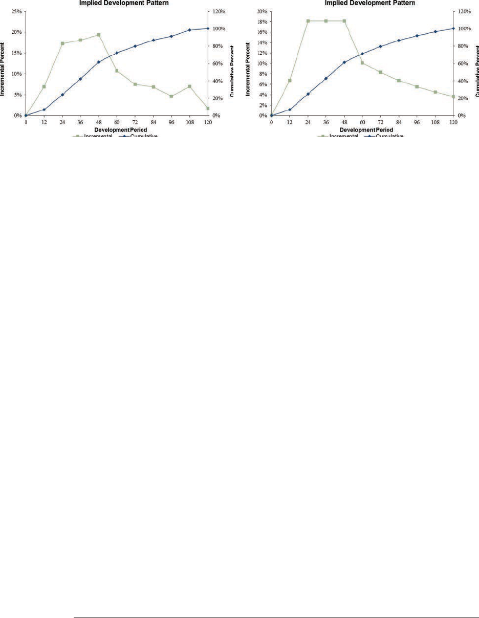
Casualty Actuarial Society 41
Using the ODP Bootstrap Model: A Practitioner’s Guide
As one nal check on the trends in this GLM bootstrap model, we can compare a
graph of the implied development patterns with the patterns from the chain ladder in
the ODP bootstrap model, as shown in Figure 5.13. Because the chain ladder model
used a parameter for each development period the implied development pattern can
appear a bit jagged, which is why it is often “smoothed” out in practice by selecting
development factors. Interestingly, the GLM bootstrap model looks quite similar,
yet with much smoother trends in the development patterns. As noted earlier, the
last GLM bootstrap development (and calendar trend) parameter can be assumed to
extend until the projected model incremental values equal zero which could then be
compared to tail factors used in the ODP bootstrap model.
54
5.5. Model Results
Once the parameter diagnostics have been reviewed, simulations should be run for
each model. ese simulation results provide an additional diagnostic tool to aid in
evaluation of the model, as described in Section 3 of CAS Working Party (2005). As an
example, we will review the results for the Taylor and Ashe (1983) data using the ODP
bootstrap model. e estimated-unpaid results shown in Figure 5.14 were simulated
using 10,000 iterations with the hetero adjustments from Figure 5.6.
5.5.1. Estimated-Unpaid Results
It’s recommended to start a diagnostic review of the estimated unpaid results with
the standard error (standard deviation) and coecient of variation (standard error
divided by the mean), shown in Figure 5.14. Keep in mind that the standard error should
increase when moving from the oldest years to the most recent years, as the standard
errors (value scale) should follow the magnitude of the mean of unpaid estimates. In
Figure 5.14, the standard errors conform to this pattern. At the same time, the standard
error for the total of all years should be larger than any individual year.
54
Results for the GLM bootstrap model, as illustrated in Figures 5.9 through 5.12, are shown in Appendix E,
although no extrapolation was included to be consistent with the ODP bootstrap results.
Figure 5.13. Implied Development Patterns
ODP Bootstrap Model “Basic” GLM Bootstrap Model

42 Casualty Actuarial Society
Using the ODP Bootstrap Model: A Practitioner’s Guide
Also, the coecients of variation should generally decrease when moving from the
oldest years to the more recent years and the coecient of variation for all years combined
should be less than for any individual year. With the exception of the 2014 and 2015
accident years, the coecients of variation in Figure 5.14 seem to also conform,
although some random uctuations may be seen.
e main reason for the decrease in the coecient of variation has to do with the
independence in the incremental claim-payment stream. Because the oldest accident
year typically has only a few incremental payments remaining, or even just one, the
variability is nearly all reected in the coecient. For more current accident years,
random variations in the future incremental payment stream may tend to oset one
another, thereby reducing the variability of the total unpaid loss.
55
While the coecients of variation should go down, they could also start to rise
again in the most recent years, as seen in Figure 5.14 for 2014 and 2015. Such reversals
are from a couple of issues:
• With an increasing number of parameters used in the model, the parameter
uncertainty tends to increase when moving from the oldest years to the more recent
years. In the most recent years, parameter uncertainty can grow to overpower process
uncertainty, which may cause the coecient of variation to start rising again. At
a minimum, increasing parameter uncertainty will slow the rate of decrease in the
coecient of variation.
• e model may be overestimating the uncertainty in recent accident years if the
increase is signicant. In that case, another model algorithm (e.g., Bornhuetter-
Ferguson or Cape Cod) may need to be used instead of a chain-ladder model.
Keep in mind also that the standard error or coecient of variation for the total
of all accident years will be less than the sum of the standard error or coecient of
variation for the individual years. is is because the model assumes that accident years
are independent.
55
To visualize this reducing Coecient of Variation, recall that the standard deviation for the total of several
independent variables is equal to the square root of the sum of the squares.
Figure 5.14. Estimated Unpaid Model Results
Taylor & Ashe Data
Accident Year Unpaid
Paid Chain Ladder Model
Accident Mean Standard Coefficient 50.0% 75.0% 95.0% 99.0%
Year Unpaid Error of Variation Minimum Maximum Percentile Percentile Percentile Percentile
2006 - - - - - - - -
2007 94,649 96,571 102.0% (119,298) 541,054 71,176 147,232 278,360 374,056
2008 473,619 199,302 42.1% (25,494) 1,217,544 454,644 590,676 830,916 1,018,835
2009 714,763 250,044 35.0% 140,156 1,642,391 684,461 882,486 1,146,017 1,396,652
2010 981,305 271,726 27.7% 324,024 2,062,359 951,467 1,148,872 1,475,857 1,731,112
2011 1,414,007 364,527 25.8% 468,645 2,829,838 1,392,288 1,642,974 2,059,339 2,349,855
2012 2,173,552 489,442 22.5% 806,008 4,293,160 2,142,306 2,489,525 3,033,205 3,345,364
2013 3,969,749 768,637 19.4% 1,655,462 6,369,285 3,913,503 4,501,100 5,307,862 5,989,765
2014 4,317,349 887,688 20.6% 1,874,779 7,677,306 4,260,113 4,898,209 5,844,560 6,516,905
2015 4,703,420 2,176,343 46.3% 445,056 13,859,166 4,493,023 6,127,676 8,500,947 10,529,157
Totals 18,842,414 2,902,735 15.4% 11,312,275 29,464,222 18,594,140 20,734,478 23,885,153 26,388,103
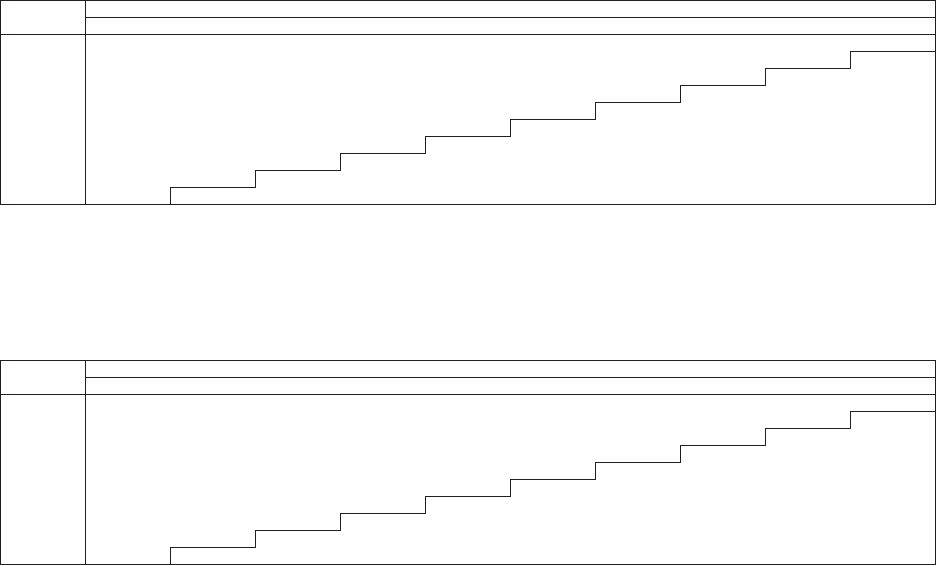
Casualty Actuarial Society 43
Using the ODP Bootstrap Model: A Practitioner’s Guide
Minimum and maximum results are the next diagnostic element in our analysis of
the estimated unpaid claims in Figure 5.14, representing the smallest and largest values
from all iterations of the simulation. ese values will need to be reviewed in order
to determine their veracity. If any of them seem implausible, the model assumptions
would need to be reviewed. eir eects could materially alter the mean indication.
Sometimes implausible extreme iterations are the result of negative incremental values
in those “rare” iterations and the limiting incremental value options discussed in
Section 4.1 can be used to constrain the model simulation process.
5.5.2. Mean, Standard Deviation and CoV of Incremental Values
e mean, standard deviation and coecients of variation for every incremental
value from the simulation process also provide useful diagnostic results, enabling us
to dig deeper into potential coecient of variation issues that may be found in the
estimated unpaid results. Consider, for example, the mean, standard deviation and
coecient of variation results shown in Figures 5.15, 5.16 and 5.17, respectively.
e mean values in Figure 5.15 appear consistent throughout and support the
increases in estimated unpaid by accident year that are shown in Figure 5.14. In fact,
the future mean values, which lay beyond the stepped diagonal line in Figure 5.15,
sum to the results in Figure 5.14. e standard deviation values in Figure 5.16 also
Taylor & Ashe Data
Accident Year Incremental Values by Development Period
Paid Chain Ladder Model
Accident Mean Values
Year 12 24 36 48 60 72 84 96 108 120+
2006 278,309 678,678 706,559 769,219 414,449 296,763 266,301 182,021 270,614 66,922
2007 380,244 940,173 979,875 1,076,297 588,887 408,707 372,144 251,228 381,983 94,649
2008 376,488 936,096 971,651 1,038,686 584,856 405,028 367,109 256,617 379,226 94,393
2009 358,750 918,068 955,061 1,023,741 565,152 405,626 367,359 249,479 372,693 92,592
2010 328,119 837,454 881,193 941,139 514,722 373,168 332,243 226,148 339,996 82,918
2011 353,894 879,226 924,325 986,018 540,281 386,069 348,473 234,329 357,224 87,913
2012 386,915 980,382 1,016,136 1,104,983 595,138 436,918 393,002 267,350 389,062 92,083
2013 477,460 1,175,498 1,227,022 1,334,527 739,306 511,050 461,997 320,655 480,476 121,737
2014 396,237 973,510 1,023,124 1,106,316 597,274 431,428 390,159 264,060 404,885 100,103
2015 342,385 875,509 913,011 977,993 539,429 389,906 344,466 230,160 347,729 85,218
Figure 5.15. Mean of Incremental Values
Taylor & Ashe Data
Accident Year Incremental Values by Development Period
Paid Chain Ladder Model
Accident Standard Error Values
Year 12 24 36 48 60 72 84 96 108 120+
2006 132,756 127,296 126,502 280,755 159,020 136,284 105,608 84,429 104,410 50,555
2007 154,318 150,888 145,947 329,237 187,519 159,277 117,183 101,220 122,902 96,571
2008 151,882 147,943 153,986 332,283 193,190 160,114 121,272 101,681 167,482 98,760
2009 146,220 150,178 149,690 327,782 186,733 158,176 119,597 125,035 171,497 98,042
2010 145,531 138,894 144,262 300,660 178,639 151,920 139,437 118,041 156,163 87,924
2011 146,339 141,271 148,740 317,044 185,534 183,768 145,838 122,161 155,734 95,224
2012 153,454 152,178 153,054 338,980 242,220 199,497 163,440 139,434 168,716 97,719
2013 173,003 165,002 168,993 447,745 261,465 215,809 165,965 141,086 201,662 121,867
2014 156,130 151,172 235,610 410,825 235,604 210,647 163,372 131,985 177,616 103,507
2015 142,319 418,523 436,805 577,315 322,537 254,332 205,111 153,930 222,174 98,010
Figure 5.16. Standard Deviation of Incremental Values
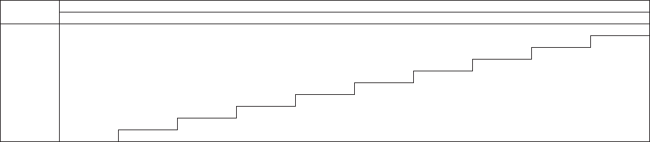
44 Casualty Actuarial Society
Using the ODP Bootstrap Model: A Practitioner’s Guide
appear consistent, although the future periods seem to have larger standard deviations
than historical periods. But the standard deviations can’t be added because the standard
deviations in Figure 5.14 represent those for aggregated incremental values by accident
year, which are less than perfectly correlated.
e dierences between the future and historical coecients of variation in
Figure 5.17 help clarify any issues with the model results. For example, notice how
the dierences by development period are more signicant in the bottom two rows in
Figure 5.17. is is consistent with the increases in the accident year 2014 and 2015
coecients of variation noted in Figure 5.14, so they can be used to diagnose the
causes noted above when compared to the same results for dierent models.
Taylor & Ashe Data
Accident Year Incremental Values by Development Period
Paid Chain Ladder Model
Accident Coefficient of Variation Values
Year 12 24 36 48 60 72 84 96 108 120+
2006 47.7% 18.8% 17.9% 36.5% 38.4% 45.9% 39.7% 46.4% 38.6% 75.5%
2007 40.6% 16.0% 14.9% 30.6% 31.8% 39.0% 31.5% 40.3% 32.2% 102.0%
2008 40.3% 15.8% 15.8% 32.0% 33.0% 39.5% 33.0% 39.6% 44.2% 104.6%
2009 40.8% 16.4% 15.7% 32.0% 33.0% 39.0% 32.6% 50.1% 46.0% 105.9%
2010 44.4% 16.6% 16.4% 31.9% 34.7% 40.7% 42.0% 52.2% 45.9% 106.0%
2011 41.4% 16.1% 16.1% 32.2% 34.3% 47.6% 41.9% 52.1% 43.6% 108.3%
2012 39.7% 15.5% 15.1% 30.7% 40.7% 45.7% 41.6% 52.2% 43.4% 106.1%
2013 36.2% 14.0% 13.8% 33.6% 35.4% 42.2% 35.9% 44.0% 42.0% 100.1%
2014 39.4% 15.5% 23.0% 37.1% 39.4% 48.8% 41.9% 50.0% 43.9% 103.4%
2015 41.6% 47.8% 47.8% 59.0% 59.8% 65.2% 59.5% 66.9% 63.9% 115.0%
Figure 5.17. Coefficient of Variation of Incremental Values

Casualty Actuarial Society 45
6. Using Multiple Models
So far we have focused only on one model. In practice, multiple stochastic models
should be used in the same way that multiple methods should be used in a deterministic
analysis. First the results for each model must be reviewed and nalized, after an
iterative process of diagnostic testing and reviewing model output to make sure the
model “ts” the data, has reasonable assumptions and produces reasonable results.
en these results can be combined by assigning a weight to the results of each model.
Two primary methods exist for combining the results for multiple models:
• Run models with the same random variables. For this algorithm, every model uses
the exact same random variables. In the “Bootstrap Models.xlsm” le, the random
values are simulated before they are used to simulate results, which means that this
algorithm may be accomplished by reusing the same set of random variables for
each model. At the end, the incremental values for each model, for each iteration
by accident year (that have a partial weight), can be weighted together.
• Run models with independent random variables. For this algorithm, every
model is run with its own random variables. In the “Bootstrap Models.xlsm” le
the random values are simulated before they are used to simulate results, which
means that this algorithm may be accomplished by simulating a new set of random
variables for each model.
56
At the end, the weights are used to randomly select a
model for each iteration by accident year so that the result is a weighted “mixture”
of models.
Both algorithms are similar to the process of weighting the results of dierent
deterministic methods to arrive at an actuarial best estimate. e process of weighting
the results of dierent stochastic models produces an actuarial best estimate of a
distribution. In practice it is also common to further “adjust” or “shift” the weighted
results by year after considering case reserves and the calculated IBNR. is “shifting”
can also be done for weighted distributions, either additively to maintain the exact
shape and width of the distribution by year or multiplicatively to maintain the exact
shape of the distribution but adjusting the width of the distribution.
56
In general, in order to simulate new random values a new seed value must be selected, otherwise the same random
values will be simulated. In the “Bootstrap Models.xlsm” le the seed value is incremented for each model and
data type so that dierent seed values are being used as long as new random numbers are generated for each
model and data type.

46 Casualty Actuarial Society
Using the ODP Bootstrap Model: A Practitioner’s Guide
e second method of combining multiple models will be illustrated using
combined Schedule P data for ve top 50 companies.
57
Data for all Schedule P lines
with 10 years of history may be found in the “Industry Data.xlsm” le, but this
example will be conned to Parts A, B, and C. For each line of business ODP bootstrap
models were run for paid and incurred data (labeled Chain Ladder), as well as paid
and incurred data for the Bornhuetter-Ferguson and Cape Cod models described in
Section3.3 and the GLM bootstrap model described in Section 3.4.
58
For this section,
only the results for Part A (Homeowners/Farmowners) will be reviewed.
59
By comparing the results for all eight models (or fewer, depending on how many are
used)
60
a qualitative assessment of the relative merits of each model may be determined.
Bayesian methods can be used to determine weighting based on the quality of each
model’s forecasts. e weights can be determined separately for each year. e table in
Figure 6.1 shows an example of weights for the Part A data.
61
e weighted results are
displayed in the “Best Estimate” column of Figure 6.2. As a parallel to a deterministic
analysis, the means from the eight models could be used to derive a reasonable range from
the modeled results (i.e., from $4,099 to $5,650) as shown in Figure 6.3. Alternatively,
if we only consider results by accident year which are given some weight when deriving
the best estimate, then the “weighted range” may be a more representative view of the
uncertainty of the actuarial central estimate.
62
When selecting weights for stochastic models, the standard deviations should also
be considered in addition to the means by model since the weighted best estimate
should reect the actuary’s judgments about the entire distribution not just a central
57
e ve companies represent large, medium and smaller companies that have been combined to maintain
anonymity. For each Part, a unique set of ve companies were used.
58
An additional benet of converting the incurred data models to a random payment stream as discussed in
Section 3.3.1 is that they can be combined with other model results.
59
Only selected weighted results are displayed and discussed in Section 6. A more complete set of results, including
results for each model, are included in Appendix A.
60
Other models in addition to the ODP bootstrap and GLM bootstrap models could also be included in the
weighting process as long as the simulated results are in the form of random incremental payment streams.
61
For simplicity, the weights are judgmental and not derived using Bayesian methods.
62
e “modeled range” in Figure 6.3 is derived using each model that is given at least some weight for any accident
year—i.e., if the model is used. In contrast, the “weighted range” is derived using only the models given weight
for each accident year, which are highlighted in grey in Figure 6.2 and 6.4.
Accide nt Model We ights by Accident Ye ar
Ye ar Paid CL Incd CL Paid BF Incd BF Paid CC Incd CC Paid GLMIncd GLMTOTAL
2006 50.0%50.0% 100.0%
2007 50.0%50.0% 100.0%
2008 50.0%50.0% 100.0%
2009 50.0%50.0% 100.0%
2010 50.0%50.0% 100.0%
2011 50.0%50.0% 100.0%
2012 50.0%50.0% 100.0%
2013 16.7%16.7% 16.7%16.7% 16.7%16.7% 100.0%
2014 16.7%16.7% 16.7%16.7% 16.7%16.7% 100.0%
2015 16.7%16.7% 16.7%16.7% 16.7%16.7% 100.0%
Figure 6.1. Model Weights by Accident Year

Casualty Actuarial Society 47
Using the ODP Bootstrap Model: A Practitioner’s Guide
estimate. us, coecients of variation by model can be used for this purpose as
illustrated in Figure 6.4.
With our focus on the entire distribution, the weights by year were used to randomly
sample the specied percentage of iterations from each model. A more complete set
of the results for the “weighted” iterations can be created similar to the tables shown
in Section 5. e companion “Best Estimate.xlsm” le can be used to weight eight
dierent models together in order to calculate a weighted best estimate. An example
for Part A is shown in the table in Figure 6.5.
As one nal check of the weighted results it would be common to review the
implied IBNR to make sure there are no issues as shown in Figure 6.6. By reviewing
this reconciliation, and perhaps also comparing it to deterministic results, additional
adjustments could be made to various assumptions. For example, from year 2006 in
Figure 6.6 it may be more realistic to revisit the tail factor assumption so that the
unpaid estimate is more consistent with the case reserves. Finally, after the interactive
process of reviewing results and adjusting assumptions is complete, it may still be
Figure 6.2. Summary of Mean Results by Model
Five Top 50 Companies
Schedule P, Part A -- Homeowners / Farmowners (in 000,000's)
Summary of Results by Model
Mean Estimated Unpaid
Accident Chain Ladder Bornhuetter Ferguson Cape Cod GLM Bootstrap Best Est.
Year Paid Incurred Paid Incurred Paid Incurred Paid Incurred (Weighted)
2006 - - - - - - - - -
2007 3 3 2 2 3 3 9 12 3
2008 41 42 28 27 32 33 27 27 41
2009 45 46 37 39 43 45 40 45 46
2010 63 62 60 59 66 71 62 73 64
2011 103 103 96 98 109 115 106 113 103
2012 222 226 169 168 191 199 213 169 224
2013 294 306 327 334 373 385 280 307 335
2014 679 723 722 753 835 871 646 650 752
2015 3,851 3,912 2,660 2,885 3,225 3,430 3,738 4,255 3,742
Totals 5,300 5,422 4,099 4,366 4,878 5,151 5,120 5,650 5,308
Five Top 50 Companies
Schedule P, Part A -- Homeowners / Farmowners (in 000,000's)
Summary of Results by Model
Ranges
Accident Best Est. Weighted Modeled
Year (Weighted) Minimum Maximum Mininum Maximum
2006 -
2007 3 3 3 2 12
2008 41 41 42 27 42
2009 46 45 46 37 46
2010 64 62 63 59 73
2011 103 103 103 96 115
2012 224 222 226 168 226
2013 335 294 385 280 385
2014 752 679 871 646 871
2015 3,742 3,225 4,255 2,660 4,255
Totals 5,308 4,674 5,992 4,099 5,650
Figure 6.3. Summary of Ranges by Accident Year

48 Casualty Actuarial Society
Five Top 50 Companies
Schedule P, Part A -- Homeowners / Farmowners (in 000,000's)
Summary of Results by Model
Coefficient of Variation
Accident Chain Ladder Bornhuetter Ferguson Cape Cod GLM Bootstrap
Year Paid Incurred Paid Incurred Paid Incurred Paid Incurred
2006
2007 264.9% 309.9% 310.2% 318.6% 276.2% 326.5% 86.4% 91.5%
2008 74.7% 101.0% 89.2% 109.3% 86.1% 95.6% 177.0% 184.0%
2009 65.5% 93.2% 69.7% 93.5% 69.2% 89.0% 119.3% 118.9%
2010 49.4% 75.6% 52.2% 78.0% 47.2% 72.7% 78.5% 78.1%
2011 34.9% 62.4% 35.7% 64.6% 33.5% 59.5% 51.3% 50.9%
2012 26.1% 49.5% 31.3% 51.4% 28.1% 50.2% 33.6% 41.5%
2013 27.3% 57.5% 26.9% 59.3% 23.3% 56.2% 27.9% 34.9%
2014 18.9% 48.8% 21.8% 51.0% 17.1% 46.7% 20.3% 26.3%
2015 9.2% 39.2% 14.4% 40.5% 8.0% 39.4% 9.0% 16.0%
Totals 8.4% 29.0% 11.1% 28.9% 7.9% 27.5% 8.7% 13.3%
Figure 6.4. Summary of CoV Results by Model
Five Top 50 Companies
Schedule P, Part A -- Homeowners / Farmowners (in 000,000’s)
Reconciliation of Total Results
Best Estimate (Weighted)
Accident Paid Incurred Case Estimate of Estimate of
Year To Date To Date Reserves IBNR Ultimate Unpaid
2006 5,234 5,237 3 (3) 5,23
4-
2007 6,470 6,479 9 (6) 6,47
33
2008 7,848 7,867 19 23 7,89
04
1
2009 7,020 7,046 26 20 7,06
64
6
2010 7,291 7,341 50 13 7,35
56
4
2011 8,134 8,225 91 12 8,23
71
03
2012 10,800 11,085 285 (61) 11,023 224
2013 7,522 7,810 28846 7,85
63
35
2014 7,968 8,703 73517 8,72
07
52
2015 9,309 12,788 3,478263 13,051 3,742
Totals 77,596 82,580 4,984324 82,905 5,308
Figure 6.6. Reconciliation of Total Results (weighted)
Five Top 50 Companies
Schedule P, Part A -- Homeowners / Farmowners (in 000,000's)
Accident Year Unpaid
Best Estimate (Weighted)
Accident Mean Standard Coefficient 50.0% 75.0% 95.0% 99.0%
Year Unpaid Error of Variation Minimum Maximum Percentile Percentile Percentile Percentile
2006 - - - - - - - -
2007 3 9 292.0% - 173 0 1 17 42
2008 41 37 88.6% - 391 32 57 111 168
2009 46 37 81.0% 1 522 36 60 114 175
2010 64 41 63.6% 4 537 55 81 139 205
2011 103 50 48.8% 10 636 94 125 193 276
2012 224 89 40.0% 36 917 211 266 382 529
2013 335 148 44.3% 25 1,460 315 401 594 865
2014 752 293 39.0% 106 2,881 725 873 1,265 1,789
2015 3,742 982 26.2% 1,094 10,700 3,654 4,118 5,392 7,059
Totals 5,308 1,044 19.7% 2,116 12,445 5,224 5,758 7,074 8,675
Normal Dist. 5,308 1,044 19.7% 5,308 6,013 7,026 7,738
logNormal Dist. 5,309 1,034 19.5% 5,211 5,935 7,158 8,164
Gamma Dist. 5,308 1,044 19.7% 5,240 5,971 7,135 8,035
TVaR 6,035 6,593 8,140 10,091
Normal TVaR 6,142 6,636 7,463 8,092
logNormal TVaR 6,121 6,691 7,780 8,733
Gamma TVaR 6,137 6,688 7,689 8,516
Figure 6.5. Estimated Unpaid Model Results (weighted)

Casualty Actuarial Society 49
Using the ODP Bootstrap Model: A Practitioner’s Guide
prudent to make adjustments to the best estimate of the unpaid by shifting the results
as noted earlier in this section. For example, since all of the models estimated the
unpaid for 2012 to be less than the case reserves, if other studies show that the case
reserves are not likely to be redundant then the actuary may decide to shift the unpaid
for 2012 so that it is at least 285.
6.1. Additional Useful Output
ree rows of percentile numbers for the normal, lognormal, and gamma distribu-
tions, which have been tted to the total unpaid-claim distribution, may be seen at the
bottom of the table in Figure 6.5. e tted mean, standard deviation, and selected
percentiles are in their respective columns; the smoothed results can be used to assess
the quality of t, parameterize a DFA model, or used to smooth the estimate of extreme
values,
63
among other applications.
Four rows of numbers indicating the Tail Value at Risk (TVaR), dened as the
average of all of the simulated values equal to or greater than the percentile value, may
also be seen at the bottom of Figure 6.5. For example, in this table, the 99th percentile
value for the total unpaid claims for all accident years combined is 8,675, while the
average of all simulated values that are greater than or equal to 8,675 is 10,091. e
Normal TVaR, Lognormal TVaR, and Gamma TVaR rows are calculated similarly,
except that they use the respective tted distributions in the calculations rather than
actual simulated values from the model.
An analysis of the TVaR values is likely to help clarify a critical issue: if the actual
outcome exceeds the X percentile value, by how much will it exceed that value on
average? is type of assessment can have important implications related to risk-based
capital calculations and other technical aspects of enterprise risk management. But it is
worth noting that the purpose of the normal, lognormal, and gamma TVaR numbers
is to provide “smoothed” values—that is, that some of the random statistical noise is
essentially prevented from distorting the calculations.
6.2. Estimated Cash Flow Results
A model’s output may also be reviewed by calendar year (or by future diagonal),
as shown in the table in Figure 6.7. A comparison of the values in Figures 6.5 and
6.7 indicates that the total rows are identical, because summing the future payments
horizontally or diagonally will produce the same total. Similar diagnostic issues (as
discussed in Section 5) may be reviewed in the table in Figure 6.7, with the exception of
the relative values of the standard errors and coecients of variation moving in opposite
directions for calendar years compared to accident years. is phenomenon makes sense
on an intuitive level when one considers that “nal” payments, projected to the furthest
point in the future, should actually be the smallest, yet relatively most uncertain.
63
A random instance of an extreme percentile can be quite erratic compared to the same percentile of a distribution
tted to the simulated distribution. is random noise for extreme percentiles could be cause for increasing the
number of iterations, but if the same percentiles for the tted distributions are stable perhaps they can be used
in lieu of more iterations. Of course the use of the extreme values assumes that the models are reliable.

50 Casualty Actuarial Society
Using the ODP Bootstrap Model: A Practitioner’s Guide
6.3. Estimated Ultimate Loss Ratio Results
Another output table, Figure 6.8, shows the estimated ultimate loss ratios by
accident year. Unlike the estimated unpaid and estimated cash-ow tables, the values
in this table are calculated using all simulated values, not just the values beyond the end
of the historical triangle. Because the simulated sample triangles represent additional
possibilities of what could have happened in the past, even as the “squaring of the
triangle” and process variance represent what could happen as those same past values
are played out into the future, we are in possession of sucient information to enable us
to estimate the variability in the loss ratio from day one until all claims are completely
paid and settled for each accident year.
64
Reviewing the simulated values indicates that the standard errors in Figure 6.8 should
be proportionate to the means, while the coecients of variation should be relatively
constant by accident year. In terms of diagnostics, any increases in standard error and
coecient of variation for the most recent years would be consistent with the reasons
Five Top 50 Companies
Schedule P, Part A -- Homeowners / Farmowners (in 000,000’s)
Calendar Year Unpaid
Best Estimate (Weighted)
Calendar Mean Standard Coefficient 50.0%75.0% 95.0%99.0%
Year Unpaid Error of Variation Minimum Maximum Percentile Percentile Percentile Percentile
2016 3,475 754 21.7% 1,297 8,4203,414 3,7974,730 5,948
2017 865 208 24.0% 293 2,148843 9821,224 1,483
2018 403 118 29.4% 115 1,298387 467614 740
2019 204 67 32.7% 56 654194 240325 412
2020 140 50 35.9% 40 539132 165233 297
2021 90 43 47.4% 12 61182112 16
92
29
2022 70 44 63.2% 6409 60 91 15
22
15
2023 51 58 112.2% -735 36 75 15
12
53
2024 10 15 146.5% -199 4154
16
7
Totals 5,308 1,044 19.7% 2,116 12,445 5,2245,758 7,0748,675
Figure 6.7. Estimated Cash Flow (weighted)
Five Top 50 Companies
Schedule P, Part A -- Homeowners / Farmowners (in 000,000’s)
Accident Year Ultimate Loss Ratios
Best Estimate (Weighted)
Accident Mean Standard Coefficient 50.0%75.0% 95.0%99.0%
Year Loss RatioError of Variation Minimum Maximum Percentile Percentile Percentile Percentile
2006 67.7% 28.5% 42.1% 0.4% 220.8% 66.1%71.1% 130.9% 158.2%
2007 79.3% 30.2% 38.1% 8.2% 262.2% 77.8%83.1% 145.5% 178.5%
2008 90.5% 31.2% 34.5% 16.9% 261.3% 89.0%94.6% 159.9% 188.9%
2009 72.8% 26.8% 36.7% 10.2% 215.6% 71.4%76.1% 131.7% 180.4%
2010 65.3% 23.3% 35.7% 10.2% 225.0% 63.8%68.0% 116.1% 139.7%
2011 64.1% 21.2% 33.1% 13.0% 190.0% 63.2%67.0% 111.8% 130.5%
2012 80.5% 24.0% 29.9% 25.0% 234.6% 79.0%83.7% 132.9% 154.6%
2013 54.7% 18.8% 34.4% 9.9% 157.7% 53.9%57.4% 96.2
%1
15.1%
2014 58.0% 19.2% 33.0% 13.0% 164.8% 57.1%60.6% 99.8
%1
18.8%
2015 88.2% 21.5% 24.4% 30.9% 232.5% 85.5%92.5% 127.9% 158.7%
Totals 71.3% 7.4% 10.4% 46.6% 112.7% 70.8%75.7% 84.4%91.7%
Figure 6.8. Estimated Loss Ratio (weighted)
64
If we are only interested in the “remaining” volatility in the loss ratio, then the values in the estimated unpaid
table (Figure 6.5) can be added to the cumulative paid values by year and divided by the premiums.

Casualty Actuarial Society 51
Using the ODP Bootstrap Model: A Practitioner’s Guide
previously cited in Section 5.4 for the estimated unpaid tables. Risk management-wise,
the loss ratio distributions have important implications for projecting pricing risk—
the mean loss ratios can be used to view any underwriting cycles and help inform the
projected mean for the next few years, while the coecients of variation can be used to
select a standard deviation for the next few years.
65
6.4. Estimated Unpaid Claim Runoff Results
Figure 6.9, shows the runo of the total unpaid claim distribution by future calendar
year. Like the estimated unpaid and estimated cash-ow tables, the values in this table
are calculated using only future simulated values, except that future diagonal results are
sequentially removed so that we are left with the remaining unpaid claims at the end of
future calendar periods. ese results are quite useful for calculating the runo of the
unpaid claim distribution when calculating risk margins using the cost of capital method.
6.5. Distribution Graphs
A nal model output to consider is a histogram of the estimated unpaid amounts
for the total of all accident years combined, as shown in the graph in Figure 6.10. e
histogram is created by counting the number of outcomes within each of 100 “buckets”
of equal size spread between the minimum and maximum outcome. To smooth the
histogram a kernel density function is often used, which is the green bars in Figure 6.10.
Another useful strategy for graphing the total unpaid distribution may be accom-
plished by creating a summary of the eight model distributions used to determine the
weighted “best estimate” and distribution. An example of this graph using the kernel
density functions is shown in Figure 6.11 and dots for the mean estimates, which
would represent a traditional range,
66
are also included.
Five Top 50 Companies
Schedule P, Part A -- Homeowners / Farmowners (in 000,000’s)
Calendar Year Unpaid Claim Runoff
Best Estimate (Weighted)
Calendar Mean Standard Coefficient 50.0% 75.0% 95.0% 99.0%
Year Unpaid Error of Variation Minimum Maximum Percentile Percentile Percentile Percentile
2015 5,308 1,044 19.7% 2,116 12,445 5,224 5,758 7,074 8,675
2016 1,834 365 19.9% 746 4,128 1,797 2,030 2,459 2,957
2017 969 218 22.5% 336 2,316 946 1,088 1,353 1,627
2018 566 146 25.8% 159 1,393 548 647 828 1,004
2019 362 114 31.5% 79 1,171 347 424 565 718
2020 222 92 41.4% 35 956 207 269 386 524
2021 132 76 57.6% 6 863 117 166 268 394
2022 62 59 96.3% (0) 745 46 84 166 269
2023 10 15 146.5% (0) 199 4154
16
7
Figure 6.9. Estimated Unpaid Claim Runoff (weighted)
65
e coecients of variation measure the variability of the loss ratios, given the movements by year. Without this
information, it is common to base the future standard deviation on the standard deviation of the historical mean
loss ratios, but this is not ideal since the variability of the mean loss ratios is not the same as the possible variation
in the actual outcomes given movements in the means.
66
A traditional range would use deterministic point estimates instead of means of the distributions, but the intent
is consistent. While the points would technically have an innitesimal probability and should therefore sit on the
x-axis, they are elevated above the zero probability level purely for illustration purposes.
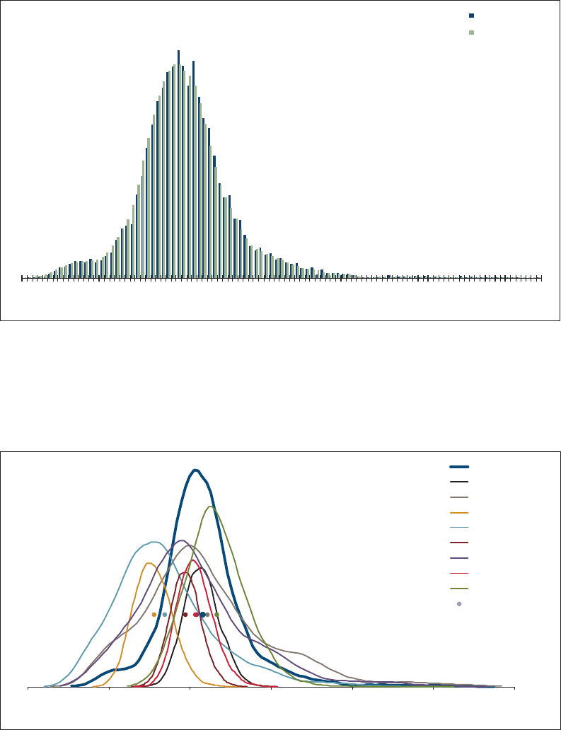
52 Casualty Actuarial Society
Using the ODP Bootstrap Model: A Practitioner’s Guide
Five Top 50 Companies
Schedule P, Part A -- Homeowners / Farmowners (in 000,000’s)
Total Unpaid Distribution
Best Estimate (Weighted)
2.1K 3.1K 4.2K 5.2K 6.2K 7.3K 8.3K 9.4K 10.4K 11.5K 12.5K
Probability
Total Unpaid
Histogram
Kernel Density
Figure 6.10. Total Unpaid Claims Distribution
Figure 6.11. Summary of Model Distributions
Five Top 50 Companies
Schedule P, Part A -- Homeowners / Farmowners (in 000,000’s)
Summary of Model Distributions
(Using Kernel Densities)
1.0K 3.0K 5.0K 7.0K 9.0K 11.0K 13.0K
Probability
Total Unpaid
Best Estimate
Paid CL
Incurred CL
Paid BF
Incurred BF
Paid CC
Incurred CC
Paid GLM
Incurred GLM
Mean Estimates

Casualty Actuarial Society 53
Using the ODP Bootstrap Model: A Practitioner’s Guide
67
For Part B and Part C, tail factors were used to illustrate the results when extrapolated beyond just squaring the
triangle. is also ows through to the Aggregate results in Appendix D.
68
is section assumes the reader is familiar with correlation.
69
It is possible to use this process with a parametric ODP bootstrap model, as described in Section 4.10, but that is
beyond the scope of the monograph.
70
For a useful reference see Kirschner, et al. (2008).
71
For example, in the “Bootstrap Models.xlsm” le the locations of the sampled residuals are shown in Step 15,
which could be replicated iteration by iteration for each business segment.
72
It is possible to ll in “missing” residuals in another segment using a randomly selected residual from elsewhere
in the triangle, but in order to maintain the same amount of correlation the selection of the other residual would
need to account for the correlation between the residuals, which complicates the process.
e corresponding tables and graphs for the Part B and Part C results are shown in
Appendices B and C, respectively.
67
6.6. Correlation
Results for an entire business unit can be estimated, after each business segment
has been analyzed and weighted into best estimates, using aggregation. is represents
another area where caution is warranted. e procedure is not a simple matter of
adding up the distributions for each segment. In order to estimate the distribution of
possible outcomes for a company as a whole, a correlation of results between segments
must be used.
68
Simulating correlated variables is commonly accomplished with a multivariate
distribution whose parameters and correlations have been previously specied. is
type of simulation is most easily applied when distributions are uniformly identical and
known in advance (for example, all derived from a multivariate normal distribution).
Unfortunately, these conditions do not generally exist for the ODP bootstrap model
(or other models), as quite often the modeling process does not allow us to know
the characteristics of overall distributions in advance or combining distributions from
dierent types of models is by denition not uniformly identical and known in advance.
Indeed, as the shapes of dierent distributions are usually slightly dierent, another
approach will be needed.
69
Two useful correlation processes for the ODP bootstrap model are location mapping
(or synchronized bootstrapping) and re-sorting.
70
With location mapping, each iteration will include sampling residuals for the rst
segment and then going back to note the location in the original residual triangle of
each sampled residual.
71
Each of the other segments is sampled using the residuals at
the same locations for their respective residual triangles. us, the correlation of the
original residuals is preserved in the sampling process.
e location-mapping process is easily implemented in Excel and does not require
the need to estimate a correlation matrix. ere are, however, two drawbacks to this
process. First, it requires all of the business segments to use data triangles that are
precisely the same size with no missing values or outliers when comparing each location
of the residuals.
72
Second, the correlation of the original residuals is used in the model,
and no other correlation assumptions can be used for stress testing the aggregate results.

54 Casualty Actuarial Society
Using the ODP Bootstrap Model: A Practitioner’s Guide
73
For a useful reference see Iman and Conover (1982) or Mildenhall (2006). In the “Aggregate Estimate.xlsm” le
the Iman-Conover algorithm is used to “Generate Rank Values” on the Inputs sheet.
74
While judgment is clearly appropriate, the typical threshold is a P-value of 5%—i.e., a P-value of 5% or less
indicates the correlation is signicantly dierent than zero, while a P-value greater than 5% indicates the
correlation is not signicantly dierent than zero.
e second correlation process, re-sorting, can be accomplished with algorithms
such as Iman-Conover
73
or Copulas, among others. e primary advantages of re-sorting
include:
• e triangles for each segment may have dierent shapes and sizes,
• Dierent correlation assumptions may be employed, and
• Dierent correlation algorithms may also have other benecial impacts on the
aggregate distribution.
For example, using a t-distribution Copula with low degrees of freedom rather
than a normal-distribution Copula, will eectively “strengthen” the focus of the
correlation in the tail of the distribution, all else being equal. is type of consideration
is important for risk-based capital and other risk modeling issues.
To induce correlation among dierent segments in the ODP bootstrap model, a
calculation of the correlation matrix using Spearman’s Rank Order and use of re-sorting
based on the ranks of the total unpaid claims for all accident years combined may be
done. e calculated correlations for Parts A, B, and C based on the paid residuals after
hetero adjustments may be seen in the table in Figure 6.12. A second part of Figure 6.12
are the P-values for each correlation coecient, which are an indication of whether a cor-
relation coecient is signicantly dierent than zero as the P-value gets close to zero.
74
By reviewing the correlation coecients for each “pair” of segments, along with
the P-values, from dierent sets of correlations matrices (e.g., from paid or incurred
data before or after the hetero adjustment) judgment can be used to select a correlation
matrix assumption. As noted above, caution is warranted as these calculated correlation
matrices are limited to the data used in the calculation and the impact of other systemic
issues, such as contagion, may also need to be considered.
Using these correlation coecients, the “Aggregate Estimate.xlsm” le, and the
simulation data for Parts A, B, and C, the aggregate results for the three lines of business
Rank Correlation of Residuals after Hetero Adjustment - Paid
LOB1 23
1 1.00 0.37 0.19
2 0.37 1.00 0.24
3 0.19 0.24 1.00
P-Values of Rank Correlation of Residuals after Hetero Adjustment - Paid
LOB1 23
1 0.00 0.01 0.17
2 0.01 0.00 0.07
3 0.17 0.07 0.00
Figure 6.12. Estimated Correlation and P-values

Casualty Actuarial Society 55
Using the ODP Bootstrap Model: A Practitioner’s Guide
were calculated and summarized in the table in Figure 6.13. A more complete set of
tables for the aggregate results is shown in Appendix D.
Note that using residuals to correlate the lines of business (or other segments), as
in the location mapping method, and measuring the correlation between residuals, as
in the re-sorting method, both tend to create correlations that are close to zero. For
reserve risk, the correlation that is desired is between the total unpaid amounts for
two segments. e correlation that is being measured is the correlation between each
incremental future loss amount, given the underlying model describing the overall
trends in the data. is may or may not be a reasonable approximation.
While not the direct measure we are hoping for, keep in mind that some level of
implied correlation between lines of business will naturally occur due to correlations
between the model parameters—e.g., similarities in development parameters, so
correlation based on the correlation between the remaining random movements in
the incremental values given the model parameters (i.e., residuals) may be reasonable.
However, an example of an issue not particularly well suited to measurement via
residual correlation is contagion between lines of business—i.e., single events that
result in claims in multiple lines of business. To account for this, and to add a bit
of conservatism, the correlation assumption can be easily changed based on actuarial
judgment.
Correlation is often thought of as being much stronger than “close to zero”, but
in this case the correlation being considered is typically the loss ratio movements by
line of business. For pricing risk, the correlation that is desired is between the loss ratio
movements by accident year between two segments. is correlation is not as likely to
be close to zero, so correlation of loss ratios (e.g., for the data in Figure 6.7) is often
done with a dierent correlation assumption compared to reserving risk.
Five Top 50 Companies
Aggregate Three Lines of Business
Accident Year Unpaid
Accident Mean Standard Coefficient 50.0%75.0% 95.0%99.0%
Year UnpaidError of Variation Minimum Maximum Percentile Percentile Percentile Percentile
2006 67 25 37.9% 0186 66 83 11
01
30
2007 107 30 28.1% 25 295105 126158 185
2008 199 49 24.8% 67 622194 226285 342
2009 298 56 18.8% 123 800293 331395 457
2010 480 69 14.3% 248 959475 522599 668
2011 862 106 12.3% 503 1,561860 9231,041 1,135
2012 1,666 187 11.2% 383 2,5551,662 1,7711,985 2,148
2013 3,070 333 10.8% 1,808 6,5223,066 3,2493,649 3,928
2014 5,632 703 12.5% 2,435 8,5555,632 6,0756,801 7,326
2015 13,270 1,788 13.5% 5,217 22,660 13,262 14,348 16,180 18,011
Totals 25,650 2,080 8.1% 16,952 36,085 25,616 26,949 29,088 30,991
Normal Dist. 25,650 2,080 8.1% 25,650 27,053 29,072 30,490
logNormal Dist. 25,650 2,088 8.1% 25,566 27,006 29,222 30,885
Gamma Dist. 25,650 2,080 8.1% 25,594 27,021 29,165 30,736
Figure 6.13. Aggregate Estimated Unpaid

56 Casualty Actuarial Society
7. Model Testing
Work on testing stochastic unpaid claim estimation models is still in its infancy. Most
papers on stochastic models display results, and some even compare a few different
models, but they tend to be void of any statistical evidence regarding how well the
model in question predicts the underlying distribution. is is quite understandable
since we don’t know what the underlying distribution is, so with real data the best
we can hope for is to retrospectively test a very old data set to see how well a model
predicted the actual outcome.
75
Testing a few old data sets is better than not, but ideally we would need many simi-
lar data sets to perform meaningful tests. One recent paper authored by the General
Insurance Reserving Oversight Committee (GI ROC) in their papers for the General
Insurance Research Organizing (GIRO) conference in 2007 titled “Best Estimates and
Reserving Uncertainty” (ROC/GIRO 2007) and their updated paper in 2008 titled
“Reserving Uncertainty” (ROC/GIRO 2008) took a first step in performing more
meaningful statistical testing of a variety of models.
A large number of models were reviewed and tested in these studies, but one of the
most interesting portions of the studies were done by comparing the unpaid liability
distributions created by the Mack and ODP bootstrap model against the “true” arti-
ficially generated unpaid loss percentiles. To accomplish these tests, artificial datasets
were constructed so that all of the Mack and ODP bootstrap assumptions, respectively,
are satisfied. While the artificial datasets were recognized as not necessarily realistic, the
“true” results are known so the Working Parties were able to test to see how well each
model performed against datasets that could be considered “perfect.”
7.1. Bootstrap Model Results
To test the ODP bootstrap model, incremental losses were simulated for a 10 ×
10 square of data based on the assumptions of the ODP bootstrap model. For the 30,000
datasets simulated, the upper triangles were used and the OPD bootstrap model from
England and Verrall (1999; 2002) were used to estimate the expected results and various
percentiles. e proportion of simulated scenarios in which the “true” outcome exceeded
the 99th percentile of the ODP Bootstrap method’s results was around 2.6–3.1%. For the
Mack method, the “true” outcome exceeded the 99th percentile around 8–13%.
75
For example, data for accident years 1994 to 2004 could be completely settled and all results known as of 2014.
us, we could use the triangle as it existed at year end 2004 to test how well a model predicted the final results.
Casualty Actuarial Society 57
Using the ODP Bootstrap Model: A Practitioner’s Guide
us, the ODP bootstrap model performed better than the Mack model for “per-
fect” data, even though the results for both models were somewhat deficient in the
sense that they both seem to under-predict the extremes of the “true” distribution. In
fairness, it should be noted however, that the ODP bootstrap model that was tested did
not include many of the “advancements” described in Section 3.2.
7.2. Future Testing
e testing done for GIRO was a significant improvement over simply looking at
results for different models, without knowing anything about the “true” underlying dis-
tribution. e next step in the testing process will be to test models against “true” results
for realistic data instead of “perfect” data. e CAS Loss Simulation Model Working
Party (2011) has created a model that will create datasets from the claim transaction
level up. e goal is to create thousands of datasets based on characteristics of real data
that can be used for testing various models.
58 Casualty Actuarial Society
8. Future Research
With testing of stochastic models in its infancy, much work in the area of future research
is needed. Only a few such areas are offered here.
• Expand testing of the ODP bootstrap model with realistic data using the CAS loss
simulation model.
• Research on how the adjustments to the ODP bootstrap and GLM bootstrap sug-
gested in this monograph perform relative to realistic data—i.e., is there a significant
improvement in the predictive power of the model given the different model con-
figurations and adjustments.
• Expand or change the ODP bootstrap model in other ways, for example use of the
Munich chain ladder (Quarg and Mack 2008) or Berquist-Sherman (1977) method
with an incurred/paid set of triangles, or the use of claim counts and average severi-
ties. Other examples could include the use of different residuals, such as deviance or
Anscombe residuals noted in Section 3.2.
• Research the use of a Bayesian or other approach to selecting weights for different
models by accident year to improve the process of combining multiple models dis-
cussed in Section 6.
• Research other risk analysis measures and how the ODP bootstrap model can be
used for enterprise risk management.
• Research how the ODP bootstrap model can be used for Solvency II requirements
in Europe and the International Accounting Standards.
• Research into the most difficult parameter to estimate: the correlation matrix.
Casualty Actuarial Society 59
9. Conclusions
While this monograph endeavored to show how the ODP bootstrap model can be
used in a variety of practical ways, and to illustrate the diagnostic tools the actuary
needs to assess whether the model is working well, it should not be assumed that the
ODP bootstrap model is well suited for every data set. However, it is hoped that the
ODP bootstrap and GLM bootstrap “toolsets” can become an integral part of
the actuaries regular estimation of unpaid claim liabilities, rather than just a “black
box” to be used only if necessary or after the deterministic methods have been used
to select a point estimate. Finally, the modeling framework allows the actuary to “fit”
the model to the data instead of simply accepting the model as is and essentially forcing
the data to “fit” the model.
60 Casualty Actuarial Society
e author gratefully acknowledges the many authors listed in the References (and
others not listed) that contributed to the foundation of the ODP bootstrap model,
without which this research would not have been possible. He also wishes to thank the
co-author of the predecessor paper, Jessica Leong, for all her support and the contri-
butions that led to this revised monograph. He would also like to thank all the peer
reviewers, Stephen Finch, Roger Hayne, Stephen Lienhard, John Major, Mark Mulvaney
and Ben Zehnwirth, who helped to improve the quality of the monograph in a vari-
ety of ways. In particular, Stephen Finch is noteworthy for keeping his wits during
an intoxicating discussion which led to the creation of the term “heteroecthesious”
data. Finally, he is grateful to the CAS referees for their comments which also greatly
improved the quality of the monograph.
Acknowledgments
Casualty Actuarial Society 61
T here are sever
al companion files designed to give the reader a deeper understanding of
the concepts discussed in the monograph. T he files are all in the “A Practitioners
Guide. zip” file at https://www.casact.org/sites/default/files/2021-02/
practitionerssuppl-shaplandmonograph04.zip T he files are:
Model Instructions.pdf—this file contains a written description of how to use the primary
bootstrap modeling files.
Primary bootstrap modeling iles:
Industry Data.xls—this file contains Schedule P data by line of business for the entire
U.S.
industry and five of the top 50 companies, for each LOB that has 10 years of data.
Bootstrap Models.xlsm—this file contains the detailed model steps described in this
m
onograph as well as various modeling options and diagnostic tests. Data can
be entered and simulations run and saved for use in calculating a weighted best
estimate.
Best Estimate
.xlsm—this file can be used to weight the results from eight different
models to get a “best estimate” of the distribution of possible outcomes.
Aggregate Estimate.xlsm—this file can be used to correlate the best estimate results
from 3 LOBs/segments.
Correlation Ranks.xlsm—this file contains examples of ranks used to correlate results
by LOB/segment.
Simple example calculation files:
GLM Framework.xlsm—this file illustrates the calculation of the GLM bootstrap
model (framework) and the corresponding ODP bootstrap model for a simple
3 × 3 triangle using (3.8).
GLM Framework C.xlsm—this file illustrates the calculation of the GLM bootstrap
m
odel (framework) and the corresponding ODP bootstrap model for a simple
3 × 3 triangle using (3.7).
GLM Framework 6.xlsm—this file illustrates the calculation of the GLM bootstrap
model (framework) and the corresponding ODP bootstrap model for a simple
6 × 6 triangle using (3.8).
GLM Framework 6C.xlsm—this file illustrates the calculation of the GLM bootstrap
m
odel (framework) and the corresponding ODP bootstrap model for a simple
6 × 6 triangle using (3.7).
Supplementary Materials
62 Casualty Actuarial Society
Using the ODP Bootstrap Model: A Practitioner’s Guide
GLM Bootstrap 6 with Outlier.xlsm—this file illustrates how the calculation of the
GLM bootstrap for a simple 6 × 6 triangle is adjusted for an outlier. It includes
different options for adjusting the ODP bootstrap model to remove an outlier.
GLM Bootstrap 6 with 3yr avg.xlsm—this file illustrates how the calculation of the
GLM bootstrap for a simple 6 × 6 triangle is adjusted to only use the equivalent of
a three-year average (i.e., the last four diagonals).
GLM Bootstrap 6 with 1 Acc Yr Parameter.xlsm—this file illustrates the calculation of
the GLM bootstrap using only one accident year (level) parameter, a development
year trend parameter for every year and no calendar year trend parameter for a simple
6 × 6 triangle.
GLM Bootstrap 6 with 1 Dev Yr Parameter.xlsm—this file illustrates the calculation of
the GLM bootstrap using only one development year trend parameter, an accident
year (level) parameter for every year and no calendar year trend parameter for a simple
6 × 6 triangle.
GLM Bootstrap 6 with 1 Acc Yr & 1 Dev Yr Parameter.xlsm—this file illustrates the
calculation of the GLM bootstrap using only one accident year (level) parameter,
one development year trend parameter and no calendar year trend parameter for a
simple 6 × 6 triangle.
GLM 6 Bootstrap with 1 Acc Yr 1 Dev Yr & 1 Cal Yr Parameter.xlsm—this file illus-
trates the calculation of the GLM bootstrap using only one accident year (level)
parameter, one development year trend parameter and one calendar year trend
parameter for a simple 6 × 6 triangle.
Appendices
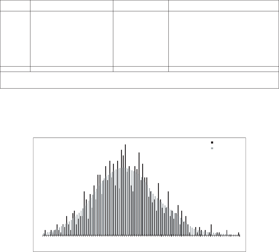
Casualty Actuarial Society 65
Appendix A—Schedule P, Part A Results
In this appendix the results for Schedule P, Part A (Homeowners/Farmowners) are shown.
Five Top 50 Companies
Schedule P, Part A -- Homeowners / Farmowners (in 000,000’s)
Total Unpaid Distribution
Paid Chain Ladder Model
4.1K 4.4K 4.7K 5.0K 5.2K 5.5K 5.8K 6.1K 6.4K 6.6K 6.9K
Probability
Total Unpaid
Histogram
Kernel Density
Figure A.2. Total Unpaid Claims Distribution (Paid Chain Ladder)
Five Top 50 Companies
Schedule P, Part A -- Homeowners / Farmowners (in 000,000's)
Accident Year Unpaid
Paid Chain Ladder Model
Accident Mean Standard Coefficient50.0% 75.0%95.0% 99.0%
Year Unpaid Error of Variation MinimumMaximum Percentile Percentile Percentile Percentile
2006 -- -
-----
2007 37264.9% -81021
73
3
2008 41 31 74.7% -204 35 59 10
01
31
2009 45 30 65.5% 7209 38 61 10
41
37
2010 63 31 49.4% 15 2135680118 161
2011 103 36 34.9% 36 28696122 17
02
13
2012 222 58 26.1% 93 497216 258328 376
2013 294 80 27.3% 126 671285 342440 513
2014 679 128 18.9% 366 1,190675 758894 1,003
2015 3,851 356 9.2% 2,675 5,0513,831 4,0754,496 4,790
Totals 5,300 447 8.4% 4,132 6,9075,282 5,5796,056 6,421
Normal Dist. 5,300 447 8.4% 5,3005,602 6,03
66
,341
logNormal Dist. 5,300 448 8.4% 5,2825,591 6,06
76
,426
Gamma Dist. 5,300 447 8.4% 5,2885,595 6,05
76
,396
Figure A.1. Estimated Unpaid Model Results (Paid Chain Ladder)
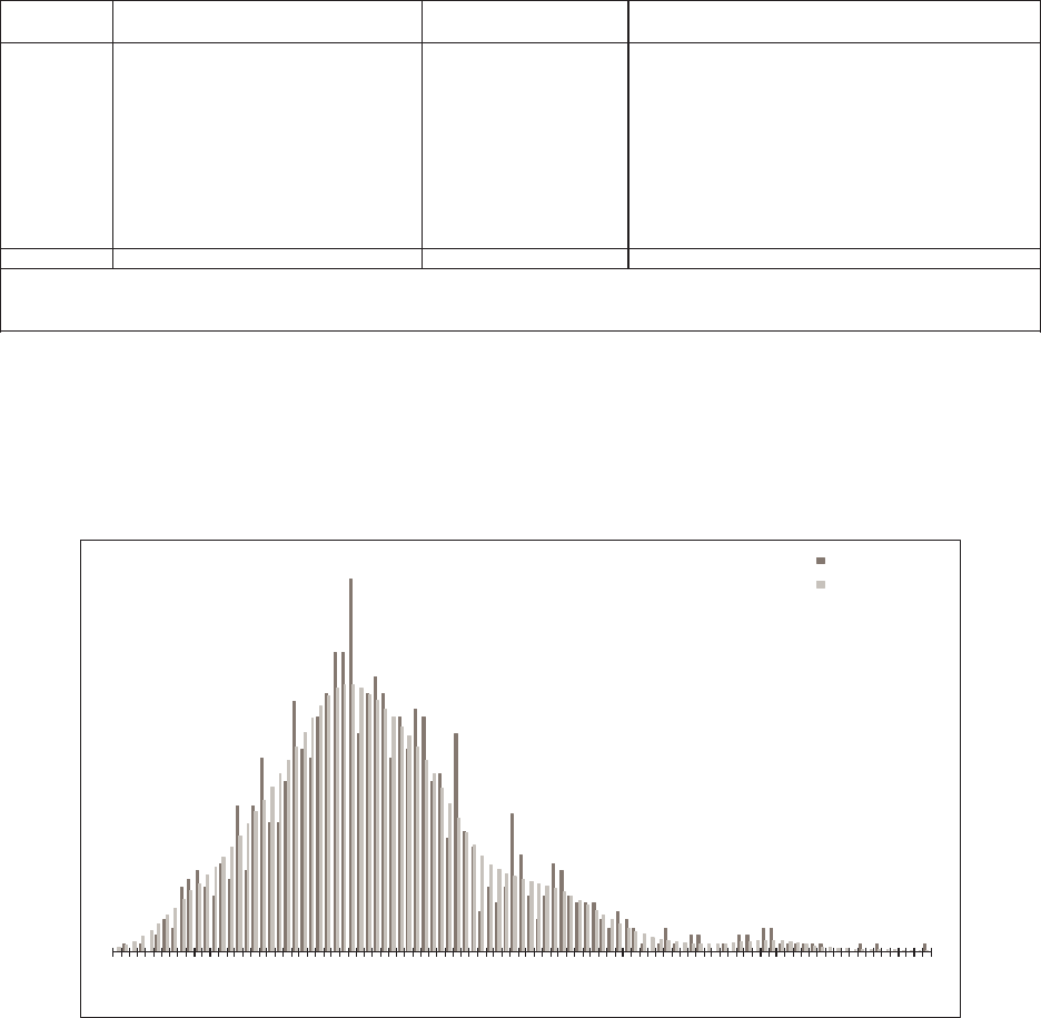
66 Casualty Actuarial Society
Using the ODP Bootstrap Model: A Practitioner’s Guide
Five Top 50 Companies
Schedule P, Part A -- Homeowners / Farmowners (in 000,000’s)
Accident Year Unpaid
Incurred Chain Ladder Model
Accident Mean Standard Coefficient50.0% 75.0%95.0% 99.0%
Year Unpaid Error of Variation MinimumMaximum Percentile Percentile Percentile Percentile
2006 -- -
-----
2007 39309.9% -93011
74
8
2008 42 42 101.0% -306 30 56 12
61
89
2009 46 42 93.2% 1325 33 57 13
52
05
2010 62 47 75.6% 4355 52 83 14
92
53
2011 103 64 62.4% 12 47389129 23
13
38
2012 226 112 49.5% 43 984202 276435 587
2013 306 176 57.5% 36 1,449271 384621 860
2014 723 353 48.8% 109 2,452664 8841,418 1,842
2015 3,912 1,534 39.2% 1,306 10,236 3,6944,523 6,70
89
,175
Totals 5,422 1,575 29.0% 1,981 12,631 5,2176,144 8,19
71
0,612
Normal Dist. 5,422 1,575 29.0% 5,4226,485 8,01
39
,086
logNormal Dist. 5,423 1,569 28.9% 5,2096,307 8,30
51
0,076
Gamma Dist. 5,422 1,575 29.0% 5,2716,386 8,24
69
,741
Figure A.3. Estimated Unpaid Model Results (Incurred Chain Ladder)
Five Top 50 Companies
Schedule P, Part A -- Homeowners / Farmowners (in 000,000’s)
Total Unpaid Distribution
Incurred Chain Ladder Model
1.9K 3.0K 4.1K 5.2K 6.2K 7.3K 8.4K 9.5K 10.5K 11.6K 12.7K
Probability
Total Unpaid
Histogram
Kernel Density
Figure A.4. Total Unpaid Claims Distribution (Incurred Chain Ladder)
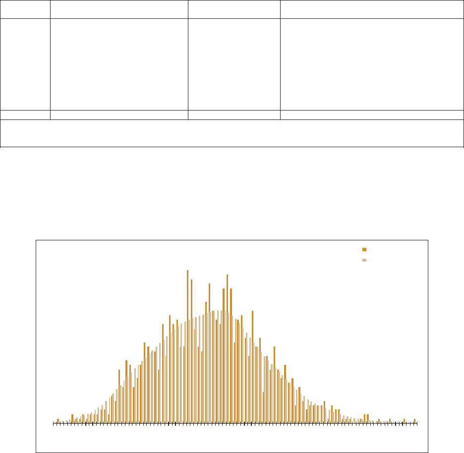
Casualty Actuarial Society 67
Using the ODP Bootstrap Model: A Practitioner’s Guide
Five Top 50 Companies
Schedule P, Part A -- Homeowners / Farmowners (in 000,000’s)
Accident Year Unpaid
Paid Bornhuetter-Ferguson Model
Accident Mean Standard Coefficient50.0% 75.0%95.0% 99.0%
Year Unpaid Error of Variation MinimumMaximum Percentile Percentile Percentile Percentile
2006 -- -
-----
2007 26310.2% -48001
03
3
2008 28 25 89.2% -188 21 40 71 115
2009 37 26 69.7% 5152 30 51 87 115
2010 60 31 52.2% 11 1865376127 153
2011 96 34 35.7% 32 27489114 16
31
94
2012 169 53 31.3% 60 367161 201269 308
2013 327 88 26.9% 115 804319 384483 573
2014 722 157 21.8% 332 1,314708 826997 1,129
2015 2,660 383 14.4% 1,689 3,8872,645 2,9083,340 3,659
Totals 4,099 456 11.1% 2,835 5,7894,096 4,3924,849 5,218
Normal Dist. 4,099 456 11.1% 4,0994,407 4,85
05
,161
logNormal Dist. 4,099 458 11.2% 4,0744,392 4,89
45
,280
Gamma Dist. 4,099 456 11.1% 4,0824,397 4,87
75
,235
Figure A.5. Estimated Unpaid Model Results (Paid Bornhuetter-Ferguson)
Five Top 50 Companies
Schedule P, Part A -- Homeowners / Farmowners (in 000,000’s)
Total Unpaid Distribution
Paid Bornhuetter-Ferguson Model
2.8K 3.1K 3.4K 3.7K 4.0K 4.3K 4.6K 4.9K 5.2K 5.5K 5.8K
Probability
Total Unpaid
Histogram
Kernel Density
Figure A.6. Total Unpaid Claims Distribution (Paid Bornhuetter-Ferguson)
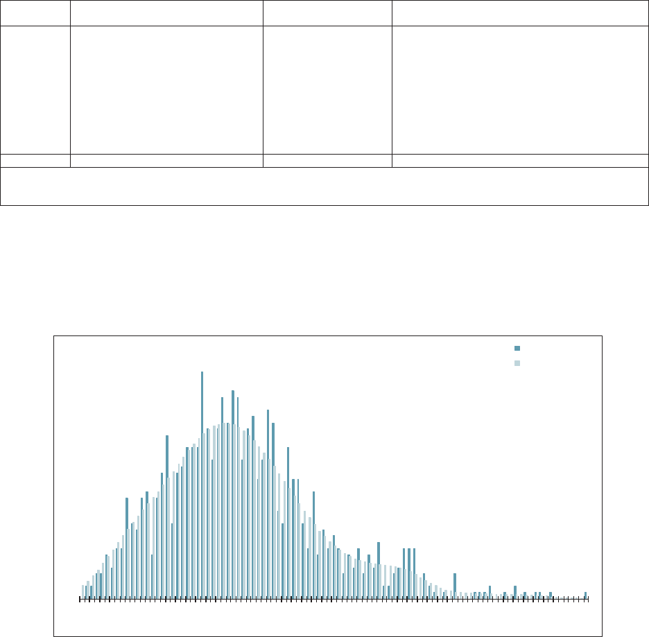
68 Casualty Actuarial Society
Using the ODP Bootstrap Model: A Practitioner’s Guide
Five Top 50 Companies
Schedule P, Part A -- Homeowners / Farmowners (in 000,000's)
Accident Year Unpaid
Incurred Bornhuetter-Ferguson Model
Accident Mean StandardCoefficient 50.0%75.0% 95.0%99.0%
Year Unpaid Error of Variation Minimum Maximum Percentile Percentile Percentile Percentile
2006 --
------
2007 27318.6% -67011
34
1
2008 27 30 109.3% -234 18 37 84 142
2009 39 36 93.5% 1263 28 50 11
41
80
2010 59 46 78.0% 4397 47 78 14
92
14
2011 98 63 64.6% 9473 84 123221 302
2012 168 86 51.4% 30 659152 210340 443
2013 334 198 59.3% 34 2,310304 412690 972
2014 753 384 51.0% 111 3,131688 9191,513 1,883
2015 2,885 1,168 40.5% 921 7,6782,699 3,4495,198 6,483
Totals 4,366 1,260 28.9% 1,873 9,8044,224 5,0486,860 8,182
Normal Dist. 4,366 1,260 28.9% 4,3665,216 6,43
87
,297
logNormal Dist. 4,367 1,272 29.1% 4,1935,083 6,70
48
,143
Gamma Dist. 4,366 1,260 28.9% 4,2465,137 6,6247,817
Figure A.7. Estimated Unpaid Model Results (Incurred Bornhuetter-Ferguson)
Five Top 50 Companies
Schedule P, Part A -- Homeowners / Farmowners (in 000,000's)
Total Unpaid Distribution
Incurred Bornhuetter-Ferguson Model
1.9K 2.7K 3.5K 4.3K 5.0K 5.8K 6.6K 7.4K 8.2K 9.0K 9.8K
Probability
Total Unpaid
Histogram
Kernel Density
Figure A.8. Total Unpaid Claims Distribution (Incurred Bornhuetter-Ferguson)
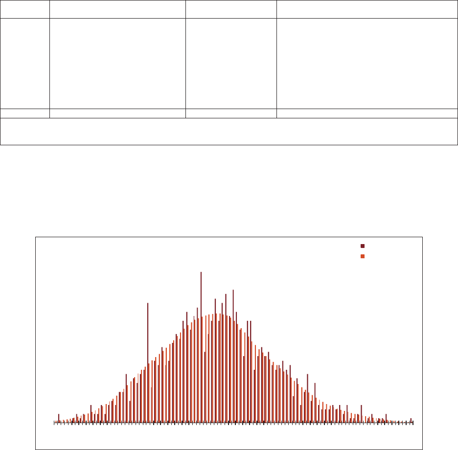
Casualty Actuarial Society 69
Using the ODP Bootstrap Model: A Practitioner’s Guide
Five Top 50 Companies
Schedule P, Part A -- Homeowners / Farmowners (in 000,000's)
Accident Year Unpaid
Paid Cape Cod Model
2006 --
------
2007 37276.2% -59011
73
8
2008 32 28 86.1% -178 25 45 89 125
2009 43 30 69.2% 6259 36 59 97 137
2010 66 31 47.2% 16 2255985122 166
2011 109 36 33.5% 43 283102 130176 213
2012 191 54 28.1% 74 401184 226288 337
2013 373 87 23.3% 156 719366 424525 600
2014 835 143 17.1% 407 1,520832 9211,082 1,192
2015 3,225 258 8.0% 2,384 4,0983,227 3,3893,659 3,855
Totals 4,878 384 7.9% 3,823 6,1744,871 5,1165,528 5,836
Normal Dist. 4,878 384 7.9% 4,8785,137 5,51
05
,772
logNormal Dist. 4,878 385 7.9% 4,8635,128 5,53
65
,841
Gamma Dist. 4,878 384 7.9% 4,8685,132 5,52
75
,816
Accident Mean StandardCoefficient 50.0%75.0% 95.0%99.0%
Year Unpaid Error of Variation Minimum Maximum Percentile Percentile PercentilePercentile
Figure A.9. Estimated Unpaid Model Results (Paid Cape Cod)
Five Top 50 Companies
Schedule P, Part A -- Homeowners / Farmowners (in 000,000's)
Total Unpaid Distribution
Paid Cape Cod Model
3.8K 4.1K 4.3K 4.5K 4.8K 5.0K 5.2K 5.5K 5.7K 5.9K 6.2K
Probability
Total Unpaid
Histogram
Kernel Density
Figure A.10. Total Unpaid Claims Distribution (Paid Cape Cod)
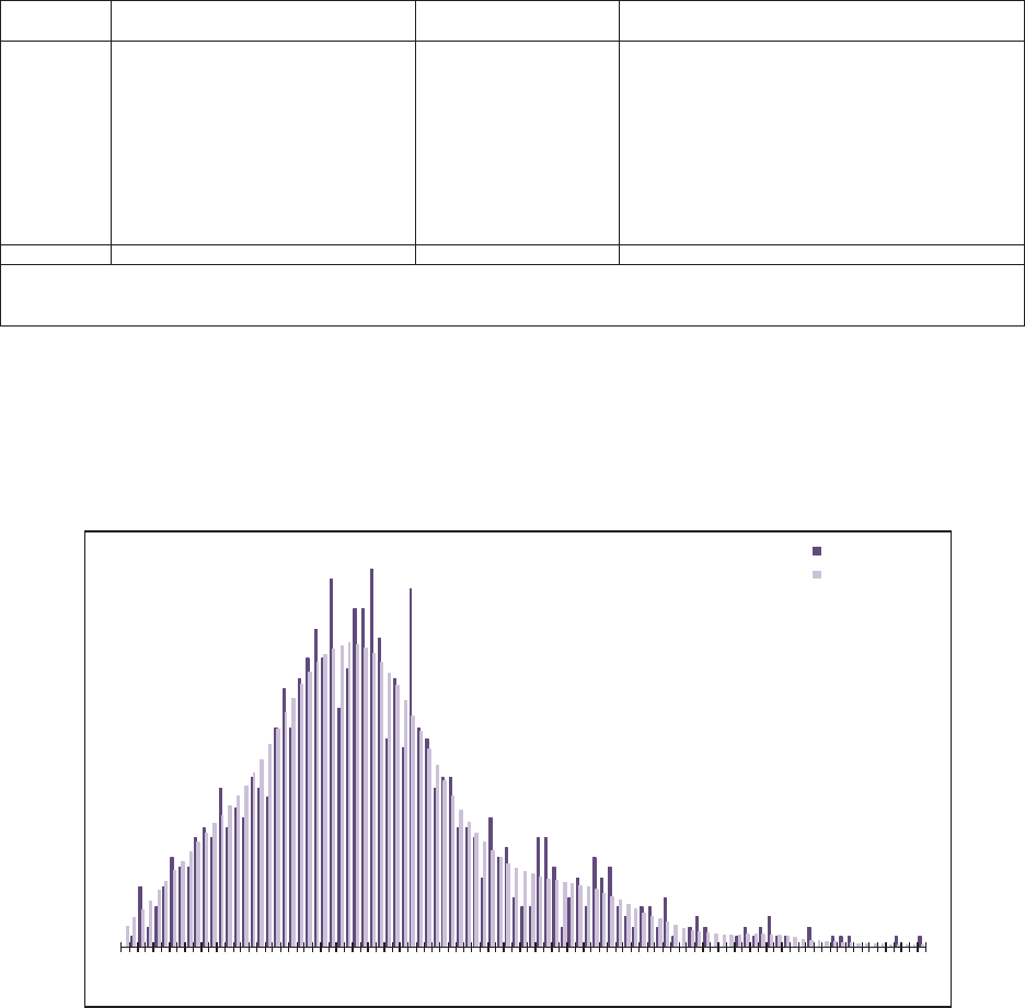
70 Casualty Actuarial Society
Using the ODP Bootstrap Model: A Practitioner’s Guide
Five Top 50 Companies
Schedule P, Part A -- Homeowners / Farmowners (in 000,000's)
Accident Year Unpaid
Incurred Cape Cod Model
Accident Mean StandardCoefficient 50.0%75.0% 95.0%99.0%
Year Unpaid Error of Variation Minimum Maximum Percentile Percentile Percentile Percentile
2006 - - - - - - - -
2007 3 10 326.5% - 117 0 1 17 50
2008 33 31 95.6% - 213 24 46 91 148
2009 45 40 89.0% 1 317 33 61 122 184
2010 71 52 72.7% 3 375 58 91 174 251
2011 115 68 59.5% 16 512 102 146 242 366
2012 199 100 50.2% 31 933 181 252 388 499
2013 385 216 56.2% 46 1,629 343 477 812 1,081
2014 871 407 46.7% 132 3,029 802 1,049 1,658 2,191
2015 3,430 1,352 39.4% 1,074 9,190 3,253 3,977 5,946 7,972
Totals 5,151 1,417 27.5% 2,424 11,216 4,972 5,790 7,785 9,512
Normal Dist. 5,151 1,417 27.5% 5,151 6,107 7,482 8,448
logNormal Dist. 5,150 1,404 27.3% 4,969 5,953 7,719 9,264
Gamma Dist. 5,151 1,417 27.5% 5,022 6,023 7,682 9,007
Figure A.11. Estimated Unpaid Model Results (Incurred Cape Cod)
Five Top 50 Companies
Schedule P, Part A -- Homeowners / Farmowners (in 000,000's)
Total Unpaid Distribution
Incurred Cape Cod Model
2.4K 3.3K 4.2K 5.0K 5.9K 6.8K 7.7K 8.6K 9.5K 10.4K 11.3K
Probability
Total Unpaid
Histogram
Kernel Density
Figure A.12. Total Unpaid Claims Distribution (Incurred Cape Cod)
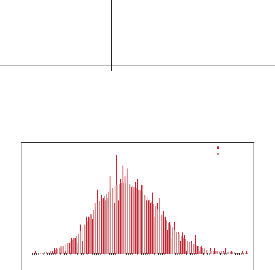
Casualty Actuarial Society 71
Using the ODP Bootstrap Model: A Practitioner’s Guide
Five Top 50 Companies
Schedule P, Part A -- Homeowners / Farmowners (in 000,000's)
Accident Year Unpaid
Paid GLM Bootstrap Model
Accident Mean StandardCoefficient 50.0%75.0% 95.0%99.0%
Year Unpaid Error of Variation Minimum Maximum Percentile Percentile Percentile Percentile
2006 - - - - - - - -
2007 9 8 86.4% 0 53 7 13 24 32
2008 27 47 177.0% 0 436 12 24 109 253
2009 40 48 119.3% 2 537 27 44 117 270
2010 62 49 78.5% 11 525 51 69 136 287
2011 106 54 51.3% 31 559 94 117 202 347
2012 213 72 33.6% 79 731 201 242 333 455
2013 280 78 27.9% 100 707 271 325 418 507
2014 646 131 20.3% 337 1,368 634 730 871 979
2015 3,738 335 9.0% 2,696 4,939 3,731 3,953 4,307 4,583
Totals 5,120 447 8.7% 3,766 6,807 5,090 5,411 5,877 6,293
Normal Dist. 5,120 447 8.7% 5,120 5,422 5,856 6,161
logNormal Dist. 5,120 446 8.7% 5,101 5,409 5,886 6,246
Gamma Dist. 5,120 447 8.7% 5,107 5,415 5,878 6,218
Figure A.13. Estimated Unpaid Model Results (Paid GLM)
Five Top 50 Companies
Schedule P, Part A -- Homeowners / Farmowners (in 000,000's)
Total Unpaid Distribution
Paid GLM Bootstrap Model
3.8K 4.1K 4.4K 4.7K 5.0K 5.3K 5.6K 5.9K 6.2K 6.5K 6.8K
Probability
Total Unpaid
Histogram
Kernel Density
Figure A.14. Total Unpaid Claims Distribution (Paid GLM)
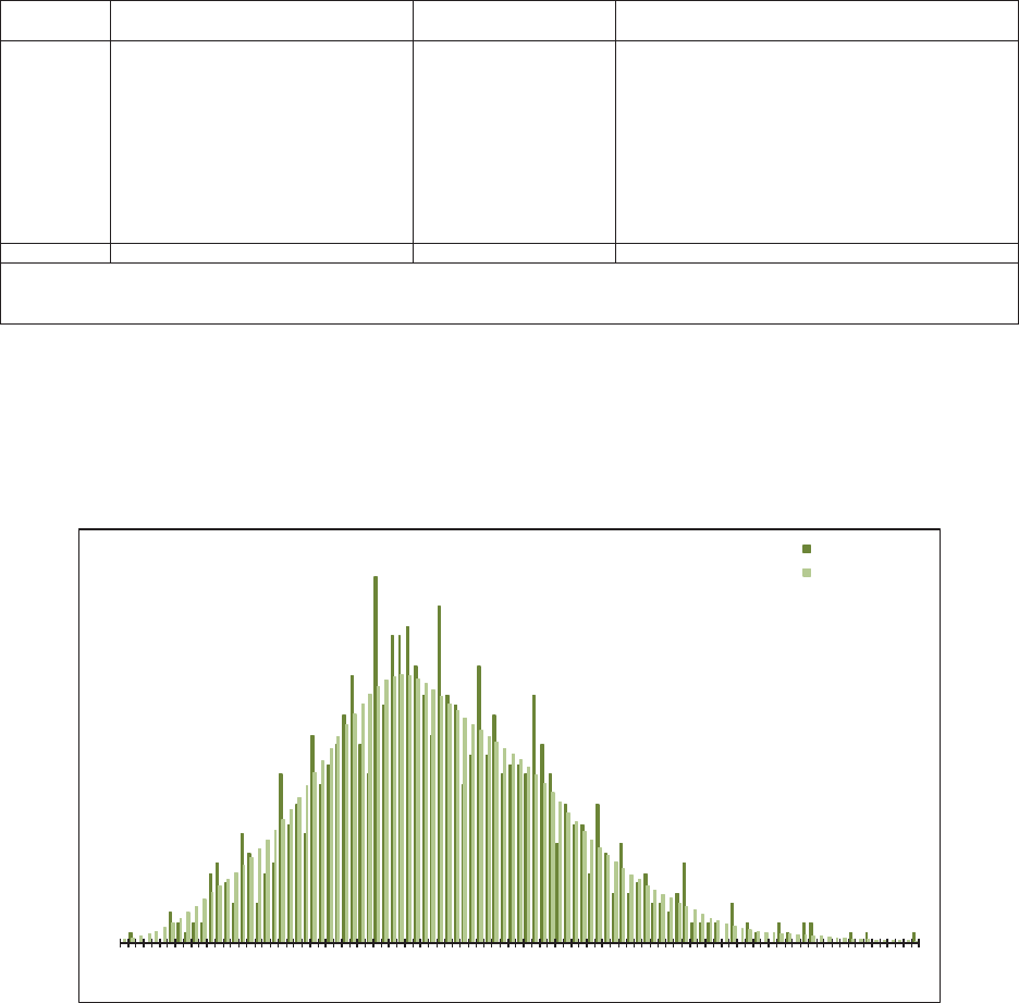
72 Casualty Actuarial Society
Using the ODP Bootstrap Model: A Practitioner’s Guide
Five Top 50 Companies
Schedule P, Part A -- Homeowners / Farmowners (in 000,000's)
Accident Year Unpaid
Incurred GLM Bootstrap Model
Accident Mean StandardCoefficient 50.0%75.0% 95.0%99.0%
Year Unpaid Error of Variation Minimum Maximum Percentile Percentile Percentile Percentile
2006 - - - - - - - -
2007 12 11 91.5% 0 66 8 16 34 48
2008 27 51 184.0% 0 520 12 25 111 262
2009 45 54 118.9% 3 678 31 52 117 268
2010 73 57 78.1% 11 892 59 85 150 301
2011 113 57 50.9% 30 771 101 128 215 360
2012 169 70 41.5% 53 712 153 198 288 415
2013 307 107 34.9% 93 1,550 293 362 491 615
2014 650 171 26.3% 280 2,713 630 743 928 1,057
2015 4,255 682 16.0% 2,581 6,888 4,216 4,670 5,413 6,295
Totals 5,650 751 13.3% 3,707 8,639 5,586 6,137 6,960 7,650
Normal Dist. 5,650 751 13.3% 5,650 6,157 6,886 7,398
logNormal Dist. 5,650 749 13.3% 5,601 6,123 6,960 7,616
Gamma Dist. 5,650 751 13.3% 5,617 6,137 6,940 7,543
Figure A.15. Estimated Unpaid Model Results (Incurred GLM)
Five Top 50 Companies
Schedule P, Part A -- Homeowners / Farmowners (in 000,000's)
Total Unpaid Distribution
Incurred GLM Bootstrap Model
3.7K 4.2K 4.7K 5.2K 5.7K 6.2K6.7K7.2K7.7K8.1
K8
.6K
Probability
Total Unpaid
Histogram
Kernel Density
Figure A.16. Total Unpaid Claims Distribution (Incurred GLM)

Casualty Actuarial Society 73
Using the ODP Bootstrap Model: A Practitioner’s Guide
Accident Model Weights by Accident Year
YearPaid CL Incd CL Paid BF Incd BF Paid CC Incd CC Paid GLMIncd GLM TOTAL
2006 50.0% 50.0% 100.0%
2007 50.0% 50.0% 100.0%
2008 50.0% 50.0% 100.0%
2009 50.0% 50.0% 100.0%
2010 50.0% 50.0% 100.0%
2011 50.0% 50.0% 100.0%
2012 50.0% 50.0% 100.0%
2013 16.7% 16.7% 16.7% 16.7% 16.7% 16.7% 100.0%
2014 16.7% 16.7% 16.7% 16.7% 16.7% 16.7% 100.0%
2015 16.7% 16.7% 16.7% 16.7% 16.7% 16.7% 100.0%
Figure A.17. Model Weights by Accident Year
Five Top 50 Companies
Schedule P, Part A -- Homeowners / Farmowners (in 000,000's)
Summary of Results by Model
Mean Estimated Unpaid
Accident Chain Ladder Bornhuetter-Ferguson Cape Cod GLM Bootstrap Best Est.
Year Paid Incurred Paid Incurred PaidIncurred PaidIncurred (Weighted)
2006 - - - - - - - - -
2007 3 3 2 2 3 3 9 12 3
2008 41 42 28 27 32 33 27 27 41
2009 45 46 37 39 43 45 40 45 46
2010 63 62 60 59 66 71 62 73 64
2011 103 103 96 98 109 115 106 113 103
2012 222 226 169 168 191 199 213 169 224
2013 294 306 327 334 373 385 280 307 335
2014 679 723 722 753 835 871 646 650 752
2015 3,851 3,912 2,660 2,885 3,225 3,430 3,738 4,255 3,742
Totals 5,300 5,422 4,099 4,366 4,878 5,151 5,120 5,650 5,308
Figure A.18. Estimated Mean Unpaid by Model
Five Top 50 Companies
Schedule P, Part A -- Homeowners / Farmowners (in 000,000's)
Summary of Results by Model
Ranges
Accident Best Est. Weighted Modeled
Year (Weighted) Minimum Maximum Mininum Maximum
2006 -
2007 3 3 3 2 12
2008 41 41 42 27 42
2009 46 45 46 37 46
2010 64 62 63 59 73
2011 103 103 103 96 115
2012 224 222 226 168 226
2013 335 294 385 280 385
2014 752 679 871 646 871
2015 3,742 3,225 4,255 2,660 4,255
Totals 5,308 4,674 5,992 4,099 5,650
Figure A.19. Estimated Ranges

74 Casualty Actuarial Society
Using the ODP Bootstrap Model: A Practitioner’s Guide
Five Top 50 Companies
Schedule P, Part A -- Homeowners / Farmowners (in 000,000's)
Reconciliation of Total Results
Best Estimate (Weighted)
Accident Paid Incurred CaseEstimate of Estimate of
Year To Date To Date ReservesIBNRUltimate Unpaid
2006 5,234 5,237 3 (3) 5,234 -
2007 6,470 6,479 9 (6) 6,473 3
2008 7,848 7,867 19 23 7,890 41
2009 7,020 7,046 26 20 7,066 46
2010 7,291 7,341 50 13 7,355 64
2011 8,134 8,225 91 12 8,237 103
2012 10,800 11,085 285 (61) 11,023 224
2013 7,522 7,810 288 46 7,856 335
2014 7,968 8,703 735 17 8,720 752
2015 9,309 12,788 3,478 263 13,051 3,742
Totals 77,596 82,580 4,984 324 82,905 5,308
Figure A.20. Reconciliation of Total Results (Weighted)
Five Top 50 Companies
Schedule P, Part A -- Homeowners / Farmowners (in 000,000's)
Accident Year Unpaid
Best Estimate (Weighted)
Accident Mean Standard Coefficient 50.0% 75.0% 95.0% 99.0%
Year Unpaid Error of Variation MinimumMaximum Percentile Percentile Percentile Percentile
2006
- - - - - - - -
2007 3 9 292.0% - 173 0 1 17 42
2008 41 37 88.6% - 391 32 57 111 168
2009 46 37 81.0% 1 522 36 60 114 175
2010 64 41 63.6% 4 537 55 81 139 205
2011 103 50 48.8% 10 636 94 125 193 276
2012 224 89 40.0% 36 917 211 266 382 529
2013 335 148 44.3% 25 1,460 315 401 594 865
2014 752 293 39.0% 106 2,881 725 873 1,265 1,789
2015 3,742 982 26.2% 1,094 10,700 3,654 4,118 5,392 7,059
Totals 5,308 1,044 19.7% 2,116 12,445 5,224 5,758 7,074 8,675
Normal Dist. 5,308 1,044 19.7% 5,308 6,013 7,026 7,738
logNormal Dist. 5,309 1,034 19.5% 5,211 5,935 7,158 8,164
Gamma Dist. 5,308 1,044 19.7% 5,240 5,971 7,135 8,035
Figure A.21. Estimated Unpaid Model Results (Weighted)
Five Top 50 Companies
Schedule P, Part A -- Homeowners / Farmowners (in 000,000's)
Calendar Year Unpaid
Best Estimate (Weighted)
Calendar Mean Standard Coefficient 50.0% 75.0% 95.0% 99.0%
Year Unpaid Error of Variation Minimum Maximum Percentile Percentile Percentile Percentile
2016 3,475 754 21.7% 1,297 8,420 3,414 3,797 4,730 5,948
2017 865 208 24.0% 293 2,148 843 982 1,224 1,483
2018 403 118 29.4% 115 1,298 387 467 614 740
2019 204 67 32.7% 56 654 194 240 325 412
2020 140 50 35.9% 40 539 132 165 233 297
2021 90 43 47.4% 12 611 82 112 169 229
2022 70 44 63.2% 6 409 60 91 152 215
2023 51 58 112.2% - 735 36 75 151 253
2024 10 15 146.5% - 199 4 15 41 67
Totals 5,308 1,044 19.7% 2,116 12,445 5,224 5,758 7,074 8,675
Figure A.22. Estimated Cash Flow (Weighted)
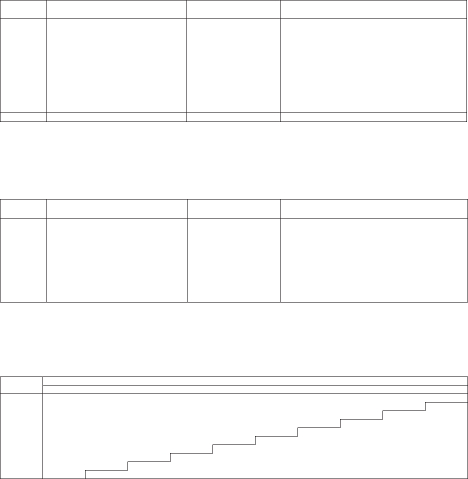
Casualty Actuarial Society 75
Using the ODP Bootstrap Model: A Practitioner’s Guide
Five Top 50 Companies
Schedule P, Part A -- Homeowners / Farmowners (in 000,000's)
Accident Year Ultimate Loss Ratios
Best Estimate (Weighted)
Accident Mean Standard Coefficient 50.0% 75.0% 95.0% 99.0%
Year Loss Ratio Error of Variation Minimum Maximum Percentile Percentile Percentile Percentile
2006 67.7% 28.5% 42.1% 0.4% 220.8% 66.1% 71.1% 130.9% 158.2%
2007 79.3% 30.2% 38.1% 8.2% 262.2% 77.8% 83.1% 145.5% 178.5%
2008 90.5% 31.2% 34.5% 16.9% 261.3% 89.0% 94.6% 159.9% 188.9%
2009 72.8% 26.8% 36.7% 10.2% 215.6% 71.4% 76.1% 131.7% 180.4%
2010 65.3% 23.3% 35.7% 10.2% 225.0% 63.8% 68.0% 116.1% 139.7%
2011 64.1% 21.2% 33.1% 13.0% 190.0% 63.2% 67.0% 111.8% 130.5%
2012 80.5% 24.0% 29.9% 25.0% 234.6% 79.0% 83.7% 132.9% 154.6%
2013 54.7% 18.8% 34.4% 9.9% 157.7% 53.9% 57.4% 96.2% 115.1%
2014 58.0% 19.2% 33.0% 13.0% 164.8% 57.1% 60.6% 99.8% 118.8%
2015 88.2% 21.5% 24.4% 30.9% 232.5% 85.5% 92.5% 127.9% 158.7%
Totals 71.3% 7.4% 10.4% 46.6% 112.7% 70.8% 75.7% 84.4% 91.7%
Figure A.23. Estimated Loss Ratio (Weighted)
Five Top 50 Companies
Schedule P, Part A -- Homeowners / Farmowners (in 000,000's)
Calendar Year Unpaid Claim Runoff
Best Estimate (Weighted)
Calendar Mean Standard Coefficient 50.0% 75.0% 95.0% 99.0%
Year Unpaid Error of Variation Minimum MaximumPercentilePercentilePercentilePercentile
2015 5,308 1,044 19.7% 2,116 12,445 5,224 5,758 7,074 8,675
2016 1,834 365 19.9% 746 4,128 1,797 2,030 2,459 2,957
2017 969 218 22.5% 336 2,316 946 1,088 1,353 1,627
2018 566 146 25.8% 159 1,393 548 647 828 1,004
2019 362 114 31.5% 79 1,171 347 424 565 718
2020 222 92 41.4% 35 956 207 269 386 524
2021 132 76 57.6% 6 863 117 166 268 394
2022 62 59 96.3% (0) 745 46 84 166 269
2023 10 15 146.5% (0) 199 4 15 41 67
Figure A.24. Estimated Unpaid Claim Runoff (Weighted)
Five Top 50 Companies
Schedule P, Part A -- Homeowners / Farmowners (in 000,000's)
Accident Year Incremental Values by Development Period
Best Estimate (Weighted)
Accident Mean Values
Year 12 24 36 48 60 72 84 96 10
81
20 +
2006 3,776 1,139 218 95 41 21 12 6 25 2
2007 4,635 1,398 268 115 51 25 15 7 31 3
2008 5,647 1,701 327 141 61 31 17 9 38 4
2009 5,065 1,525 294 126 56 28 16 8 34 3
2010 5,318 1,602 307 132 57 29 17 8 36 3
2011 5,882 1,774 340 145 64 32 18 9 40 4
2012 7,909 2,378 457 197 86 43 25 12 53 5
2013 5,589 1,683 323 156 68 35 20 10 42 4
2014 6,197 1,870 392 168 73 37 21 10 46 4
2015 9,615 2,744 521 222 92 53 33 20 47 10
Figure A.25. Mean Of Incremental Values (Weighted)
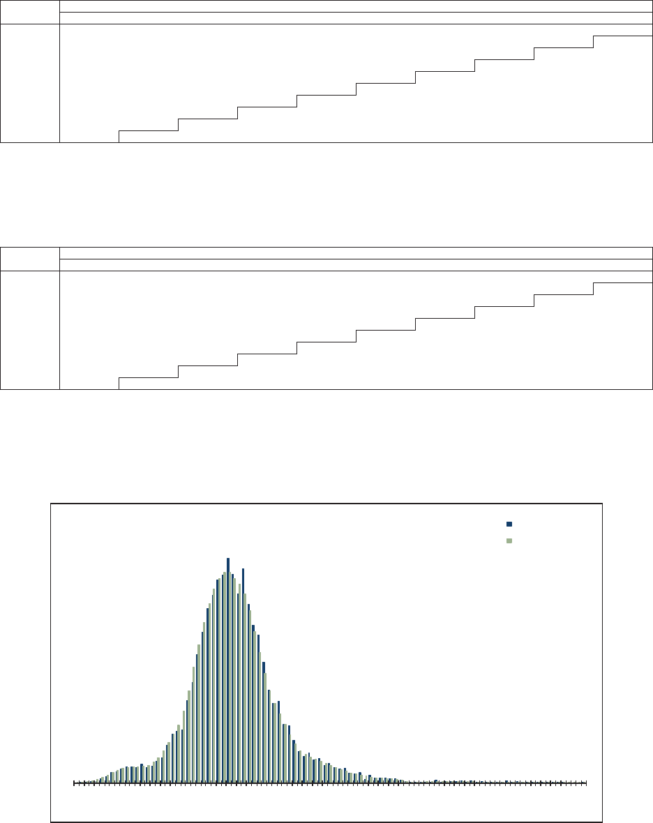
76 Casualty Actuarial Society
Using the ODP Bootstrap Model: A Practitioner’s Guide
Five Top 50 Companies
Schedule P, Part A -- Homeowners / Farmowners (in 000,000's)
Accident Year Incremental Values by Development Period
Best Estimate (Weighted)
Accident Standard Error Values
Year 12 24 36 48 60 72 84 96 10
81
20 +
2006 1,597 502 119 64 33 11 7 2 23 4
2007 1,779 550 129 68 36 12 8 3 26 9
2008 1,960 603 147 77 38 13 8 3 35 10
2009 1,873 576 139 73 38 13 8 3 34 9
2010 1,906 596 143 75 38 13 9 3 34 9
2011 1,952 610 147 76 40 14 9 3 37 10
2012 2,375 733 173 92 49 17 11 4 44 11
2013 1,938 599 142 88 45 16 10 4 38 10
2014 2,054 639 173 90 47 16 10 4 41 11
2015 2,342 727 178 101 51 20 16 13 57 15
Figure A.26. Standard Deviation of Incremental Values (Weighted)
Five Top 50 Companies
Schedule P, Part A -- Homeowners / Farmowners (in 000,000's)
Accident Year Incremental Values by Development Period
Best Estimate (Weighted)
Accident Coefficients of Variation
Year 12 24 36 48 60 72 84 96 10
81
20 +
2006 42.3%44.1% 54.4% 67.8% 80.8% 52.6% 58.8% 43.2% 89.8
%1
57.5%
2007 38.4%39.3% 48.2% 59.5% 71.1% 47.7% 52.9% 38.7% 82.4
%2
92.0%
2008 34.7%35.5% 44.8% 54.5% 62.5% 43.0% 47.9% 34.9% 92.6
%2
66.2%
2009 37.0%37.8% 47.3% 58.1% 68.6% 45.4% 50.3% 37.7% 98.4
%2
72.2%
2010 35.8%37.2% 46.5% 56.8% 66.1% 44.8% 52.4% 36.5% 95.5
%2
79.7%
2011 33.2%34.4% 43.1% 52.8% 62.4% 42.5% 49.3% 34.0% 92.6
%2
67.9%
2012 30.0%30.8% 37.8% 46.6% 57.2% 38.4% 44.6% 30.6% 82.8
%2
34.2%
2013 34.7%35.6% 43.9% 56.5% 66.6% 45.8% 51.2% 37.4% 91.1
%2
50.9%
2014 33.2%34.2% 44.2% 53.4% 64.1% 43.4% 49.6% 36.0% 88.9
%2
53.1%
2015 24.4%26.5% 34.2% 45.3% 55.8% 37.2% 47.4% 66.2% 120.2% 146.5%
Figure A.27. Coefficient of Variation of Incremental Values (Weighted)
Five Top 50 Companies
Schedule P, Part A -- Homeowners / Farmowners (in 000,000's)
Total Unpaid Distribution
Best Estimate (Weighted)
2.1K 3.1K 4.2K 5.2K 6.2K 7.3K 8.3K 9.4K 10.4K 11.5K 12.5K
Probability
Total Unpaid
Histogram
Kernel Density
Figure A.28. Total Unpaid Claims Distribution (Weighted)
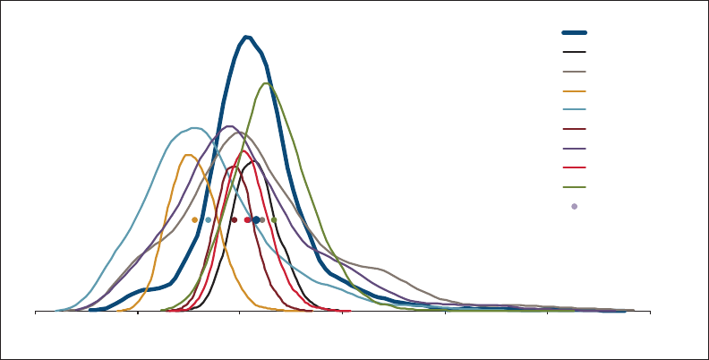
Casualty Actuarial Society 77
Using the ODP Bootstrap Model: A Practitioner’s Guide
Five Top 50 Companies
Schedule P, Part A -- Homeowners / Farmowners (in 000,000's)
Summary of Model Distributions
(Using Kernel Densities)
1.0K 3.0K 5.0K 7.0K 9.0K 11.0K 13.0K
Probability
Total Unpaid
Best Estimate
Paid CL
Incurred CL
Paid BF
Incurred BF
Paid CC
Incurred CC
Paid GLM
Incurred GLM
Mean Estimates
Figure A.29. Summary of Model Distributions
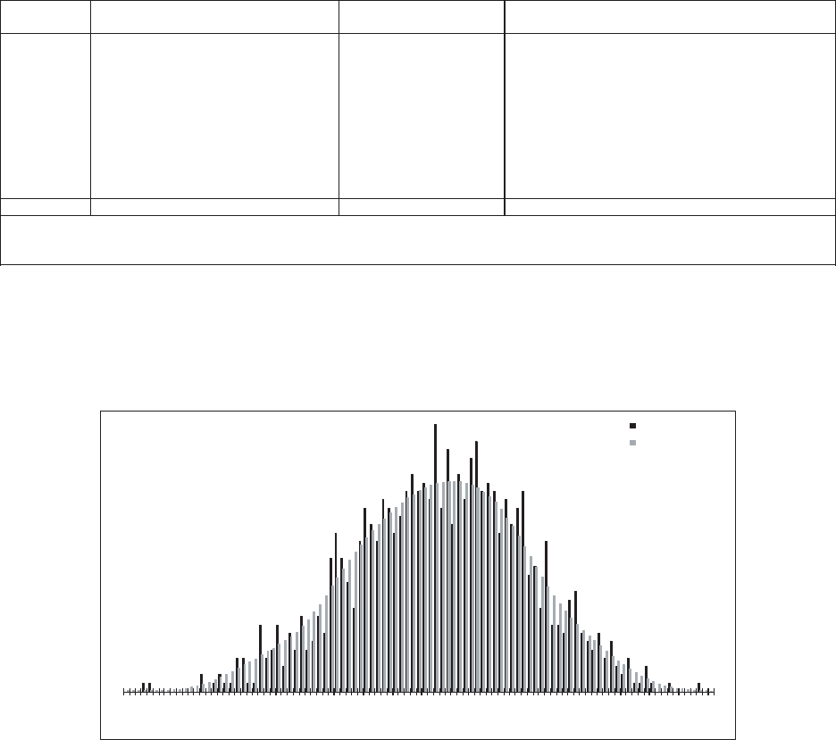
78 Casualty Actuarial Society
Appendix B—Schedule P, Part B Results
In this appendix the results for Schedule P, Part B (Private Passenger Auto Liability) are
shown.
Five Top 50 Companies
Schedule P, Part B -- Private Passenger Auto Liability (in 000,000’s)
Accident Year Unpaid
Paid Chain Ladder Model
Accident Mean Standard Coefficient 50.0% 75.0% 95.0% 99.0%
Year Unpaid Error of Variation MinimumMaximum Percentile Percentile Percentile Percentile
2006 59 23 38.8% - 125 58 75 97 112
2007 90 25 27.3% 26 164 90 107 131 147
2008 135 27 19.9% 64 217 134 153 178 196
2009 214 32 14.8% 128 322 213 237 265 289
2010 339 31 9.2% 252 443 340 361 390 413
2011 586 38 6.6% 459 707 585 610 651 687
2012 1,109 51 4.6% 949 1,281 1,108 1,144 1,191 1,226
2013 2,089 75 3.6% 1,868 2,329 2,090 2,140 2,211 2,252
2014 3,917 127 3.3% 3,457 4,357 3,919 4,002 4,129 4,203
2015 8,033 219 2.7% 7,335 8,667 8,042 8,175 8,399 8,532
Totals 16,573 385 2.3% 15,252 17,728 16,581 16,842 17,192 17,399
Normal Dist. 16,573 385 2.3% 16,573 16,833 17,207 17,469
logNormal Dist. 16,573 386 2.3% 16,569 16,831 17,216 17,491
Gamma Dist. 16,573 385 2.3% 16,570 16,831 17,212 17,482
Figure B.1. Estimated Unpaid Model Results (Paid Chain Ladder)
Five Top 50 Companies
Schedule P, Part B -- Private Passenger Auto Liability (in 000,000’s)
Total Unpaid Distribution
Paid Chain Ladder Model
15.2K 15.5K 15.7K 16.0K 16.2K 16.5K 16.7K 17.0K 17.3K 17.5K 17.8K
Probability
Total Unpaid
Histogram
Kernel Density
Figure B.2. Total Unpaid Claims Distribution (Paid Chain Ladder)
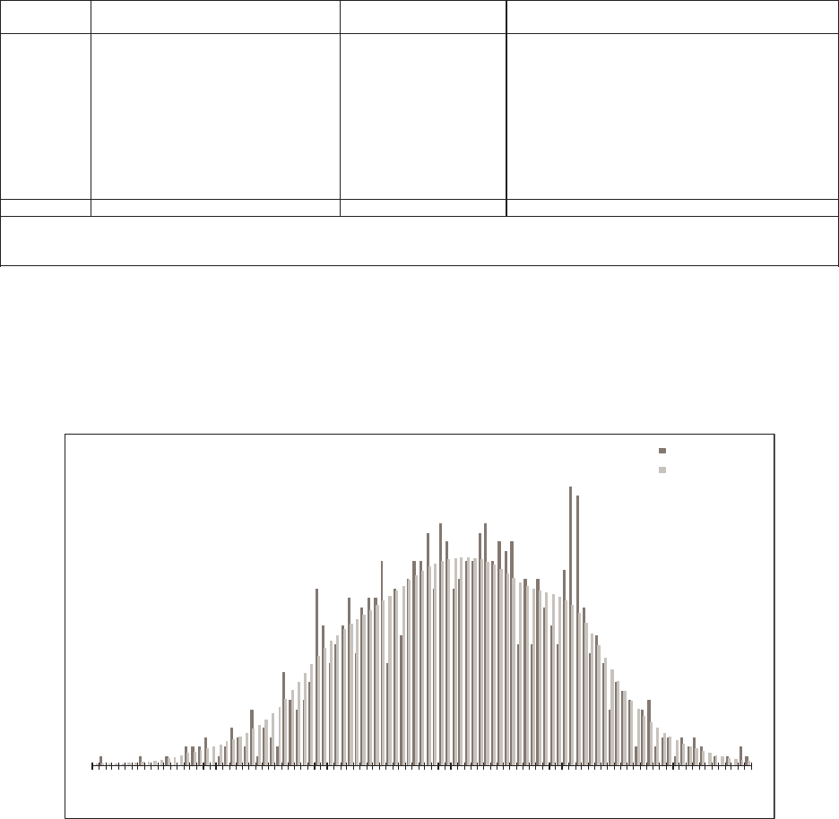
Casualty Actuarial Society 79
Using the ODP Bootstrap Model: A Practitioner’s Guide
Five Top 50 Companies
Schedule P, Part B -- Private Passenger Auto Liability (in 000,000’s)
Accident Year Unpaid
Incurred Chain Ladder Model
Accident Mean Standard Coefficient 50.0% 75.0% 95.0% 99.0%
Year Unpaid Error of Variation MinimumMaximum Percentile Percentile Percentile Percentile
2006 58 27 46.8% - 156 56 77 103 131
2007 89 31 34.9% 17 212 87 108 146 170
2008 135 37 27.5% 48 278 133 159 196 226
2009 213 46 21.8% 106 397 210 246 290 326
2010 343 63 18.4% 178 560 342 387 445 492
2011 590 106 18.0% 304 886 590 661 764 823
2012 1,125 196 17.4% 610 2,320 1,133 1,265 1,439 1,502
2013 2,133 370 17.4% 1,167 3,115 2,165 2,404 2,722 2,846
2014 4,025 680 16.9% 2,324 5,470 4,078 4,514 5,076 5,298
2015 8,343 1,369 16.4% 4,886 12,352 8,502 9,290 10,413 10,940
Totals 17,054 1,620 9.5% 11,558 21,439 17,111 18,280 19,534 20,583
Normal Dist. 17,054 1,620 9.5% 17,054 18,147 19,719 20,824
logNormal Dist. 17,055 1,653 9.7% 16,976 18,120 19,902 21,257
Gamma Dist. 17,054 1,620 9.5% 17,003 18,117 19,804 21,048
Figure B.3. Estimated Unpaid Model Results (Incurred Chain Ladder)
Five Top 50 Companies
Schedule P, Part B -- Private Passenger Auto Liability (in 000,000’s)
Total Unpaid Distribution
Incurred Chain Ladder Model
11.5K 12.5K 13.5K 14.5K 15.5K 16.5K 17.5K 18.5K 19.5K 20.5K 21.5K
Probability
Total Unpaid
Histogram
Kernel Density
Figure B.4. Total Unpaid Claims Distribution (Incurred Chain Ladder)
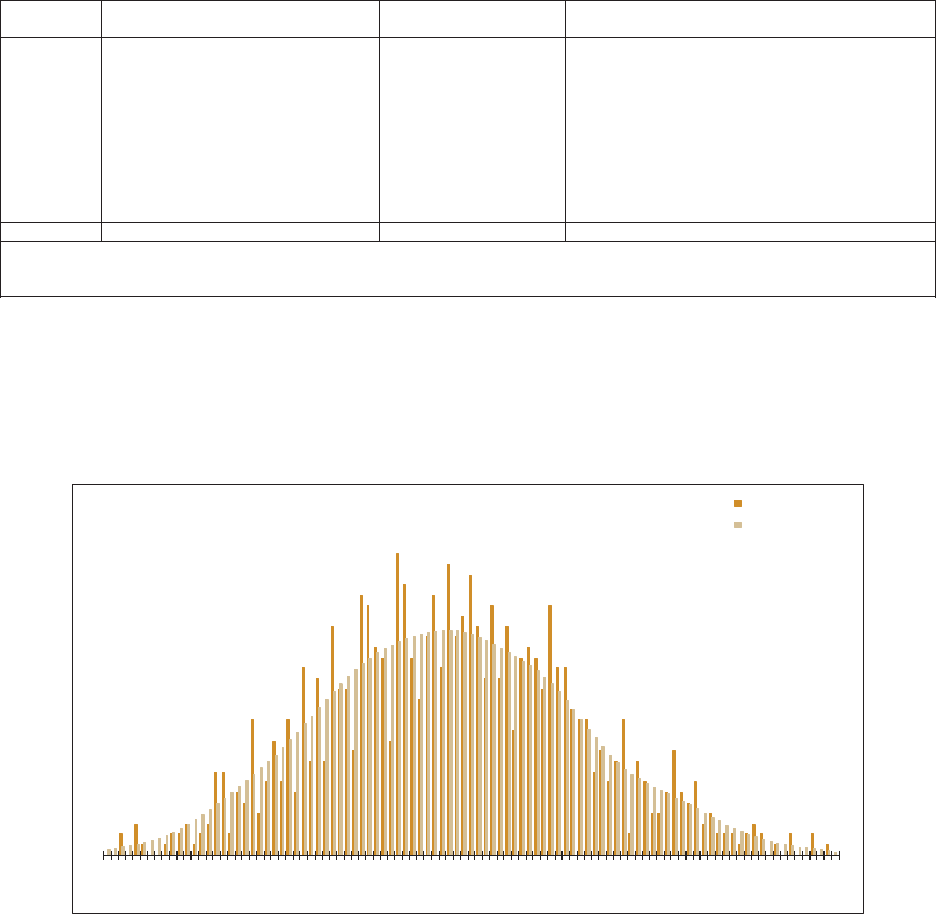
80 Casualty Actuarial Society
Using the ODP Bootstrap Model: A Practitioner’s Guide
Five Top 50 Companies
Schedule P, Part B -- Private Passenger Auto Liability (in 000,000’s)
Accident Year Unpaid
Paid Bornhuetter-Ferguson Model
Accident Mean Standard Coefficient 50.0% 75.0% 95.0% 99.0%
Year Unpaid Error of Variation MinimumMaximum Percentile Percentile Percentile Percentile
2006 54 22 40.2% - 126 54 68 91 109
2007 76 22 28.7% 22 157 77 90 112 130
2008 112 24 21.2% 52 189 112 127 154 171
2009 188 30 16.0% 97 295 188 208 238 258
2010 343 36 10.4% 227 472 343 366 404 429
2011 625 50 8.0% 459 819 624 657 709 747
2012 1,162 77 6.7% 910 1,386 1,160 1,212 1,289 1,353
2013 2,217 134 6.1% 1,855 2,666 2,215 2,312 2,450 2,536
2014 3,942 218 5.5% 3,304 4,750 3,937 4,083 4,308 4,444
2015 7,990 441 5.5% 6,885 9,426 7,988 8,271 8,763 9,066
Totals 16,709 562 3.4% 15,239 18,369 16,701 17,096 17,695 18,035
Normal Dist. 16,709 562 3.4% 16,709 17,088 17,633 18,016
logNormal Dist. 16,709 561 3.4% 16,700 17,083 17,648 18,057
Gamma Dist. 16,709 562 3.4% 16,703 17,085 17,644 18,043
Figure B.5. Estimated Unpaid Model Results (Paid Bornhuetter-Ferguson)
Five Top 50 Companies
Schedule P, Part B -- Private Passenger Auto Liability (in 000,000’s)
Total Unpaid Distribution
Paid Bornhuetter-Ferguson Model
15.2K 15.5K 15.8K 16.2K 16.5K 16.8K 17.1K 17.5K 17.8K 18.1K 18.4K
Probability
Total Unpaid
Histogram
Kernel Density
Figure B.6. Total Unpaid Claims Distribution (Paid Bornhuetter-Ferguson)
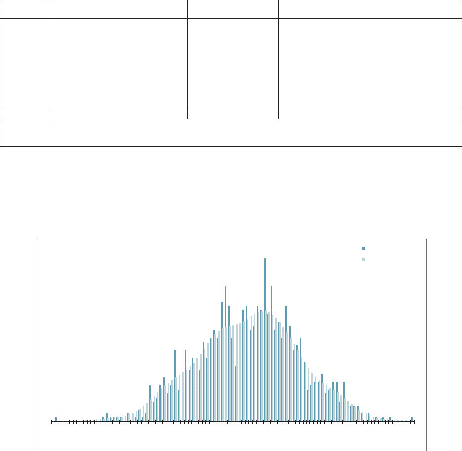
Casualty Actuarial Society 81
Using the ODP Bootstrap Model: A Practitioner’s Guide
Five Top 50 Companies
Schedule P, Part B -- Private Passenger Auto Liability (in 000,000’s)
Accident Year Unpaid
Incurred Bornhuetter-Ferguson Model
Accident Mean Standard Coefficient 50.0% 75.0% 95.0% 99.0%
Year Unpaid Error of Variation MinimumMaximum Percentile Percentile Percentile Percentile
2006 54 24 45.4% - 155 52 68 97 121
2007 76 25 33.1% 13 181 74 92 120 141
2008 111 30 27.2% 42 213 108 132 165 187
2009 188 42 22.5% 78 337 187 215 261 295
2010 344 68 19.7% 142 577 347 391 455 502
2011 627 116 18.5% 319 979 626 709 816 888
2012 1,167 217 18.6% 614 2,121 1,175 1,309 1,517 1,655
2013 2,234 420 18.8% 1,124 5,710 2,270 2,517 2,855 3,060
2014 3,997 689 17.2% 2,017 5,678 4,025 4,470 5,113 5,363
2015 8,289 1,370 16.5% 2,250 11,646 8,398 9,216 10,412 10,925
Totals 17,088 1,617 9.5% 10,942 22,273 17,177 18,198 19,785 20,539
Normal Dist. 17,088 1,617 9.5% 17,088 18,178 19,747 20,849
logNormal Dist. 17,089 1,648 9.6% 17,010 18,150 19,926 21,277
Gamma Dist. 17,088 1,617 9.5% 17,037 18,149 19,831 21,072
Figure B.7. Estimated Unpaid Model Results (Incurred Bornhuetter-Ferguson)
Five Top 50 Companies
Schedule P, Part B -- Private Passenger Auto Liability (in 000,000’s)
Total Unpaid Distribution
Incurred Bornhuetter-Ferguson Model
10.9K 12.0K 13.2K 14.3K 15.5K 16.6K 17.7K 18.9K 20.0K 21.2K 22.3K
Probability
Total Unpaid
Histogram
Kernel Density
Figure B.8. Total Unpaid Claims Distribution (Incurred Bornhuetter-Ferguson)
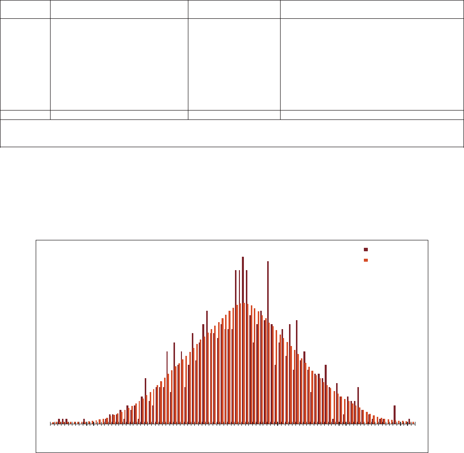
82 Casualty Actuarial Society
Using the ODP Bootstrap Model: A Practitioner’s Guide
Five Top 50 Companies
Schedule P, Part B -- Private Passenger Auto Liability (in 000,000’s)
Accident Year Unpaid
Paid Cape Cod Model
Accident Mean Standard Coefficient 50.0% 75.0% 95.0% 99.0%
Year Unpaid Error of Variation MinimumMaximum Percentile Percentile Percentile Percentile
2006 55 23 41.2% - 136 55 70 94 108
2007 80 23 28.9% 23 161 79 95 118 133
2008 117 24 20.9% 57 205 117 134 159 175
2009 196 30 15.5% 116 305 195 216 247 270
2010 354 34 9.5% 263 459 353 377 410 436
2011 642 42 6.5% 513 773 642 670 710 738
2012 1,197 54 4.5% 1,042 1,365 1,198 1,234 1,288 1,331
2013 2,292 80 3.5% 2,045 2,553 2,294 2,345 2,424 2,474
2014 4,145 118 2.9% 3,761 4,502 4,145 4,219 4,345 4,439
2015 8,598 172 2.0% 8,057 9,073 8,596 8,711 8,894 8,987
Totals 17,676 376 2.1% 16,428 18,791 17,675 17,929 18,306 18,488
Normal Dist. 17,676 376 2.1% 17,676 17,930 18,295 18,551
logNormal Dist. 17,676 377 2.1% 17,672 17,928 18,302 18,570
Gamma Dist. 17,676 376 2.1% 17,674 17,929 18,300 18,563
Figure B.9. Estimated Unpaid Model Results (Paid Cape Cod)
Five Top 50 Companies
Schedule P, Part B -- Private Passenger Auto Liability (in 000,000’s)
Total Unpaid Distribution
Paid Cape Cod Model
16.4K 16.6K 16.9K 17.1K 17.4K 17.6K 17.9K 18.1K 18.3K 18.6K 18.8K
Probability
Total Unpaid
Histogram
Kernel Density
Figure B.10. Total Unpaid Claims Distribution (Paid Cape Cod)
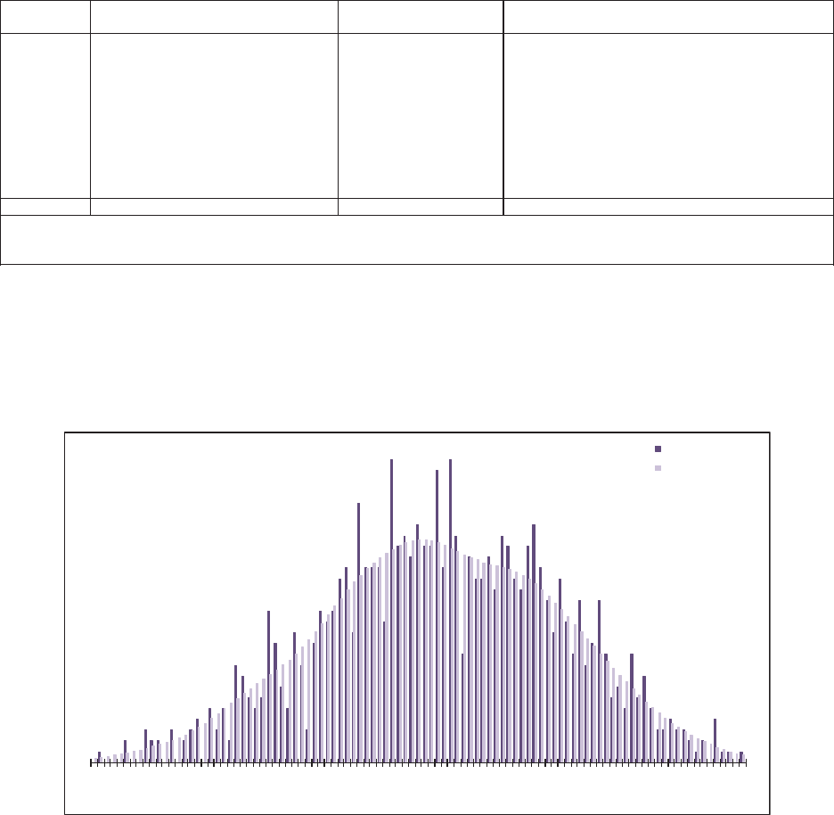
Casualty Actuarial Society 83
Using the ODP Bootstrap Model: A Practitioner’s Guide
Five Top 50 Companies
Schedule P, Part B -- Private Passenger Auto Liability (in 000,000’s)
Accident Year Unpaid
Incurred Cape Cod Model
Accident Mean Standard Coefficient 50.0% 75.0% 95.0% 99.0%
Year Unpaid Error of Variation MinimumMaximum Percentile Percentile Percentile Percentile
2006 56 24 43.7% - 133 54 71 96 114
2007 80 27 33.8% 18 175 79 98 126 147
2008 118 32 27.4% 35 230 116 138 175 203
2009 197 44 22.5% 90 351 194 228 271 309
2010 358 69 19.3% 184 544 358 407 474 509
2011 650 115 17.6% 324 953 647 730 843 900
2012 1,201 213 17.7% 675 1,697 1,224 1,352 1,534 1,632
2013 2,308 388 16.8% 1,247 3,598 2,335 2,579 2,939 3,074
2014 4,178 701 16.8% 2,248 5,709 4,247 4,697 5,271 5,516
2015 8,526 1,424 16.7% 4,605 11,643 8,725 9,508 10,707 11,151
Totals 17,672 1,677 9.5% 12,794 21,955 17,649 18,915 20,366 21,243
Normal Dist. 17,672 1,677 9.5% 17,672 18,803 20,430 21,573
logNormal Dist. 17,673 1,706 9.7% 17,591 18,772 20,610 22,008
Gamma Dist. 17,672 1,677 9.5% 17,619 18,772 20,517 21,805
Figure B.11. Estimated Unpaid Model Results (Incurred Cape Cod)
Five Top 50 Companies
Schedule P, Part B -- Private Passenger Auto Liability (in 000,000’s)
Total Unpaid Distribution
Incurred Cape Cod Model
12.7K 13.7K 14.6K 15.5K 16.4K 17.4K 18.3K 19.2K 20.1K 21.1K 22.0K
Probability
Total Unpaid
Histogram
Kernel Density
Figure B.12. Total Unpaid Claims Distribution (Incurred Cape Cod)
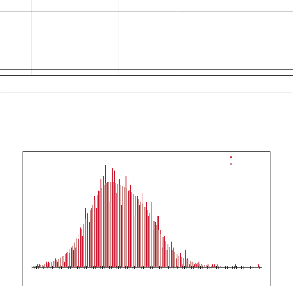
84 Casualty Actuarial Society
Using the ODP Bootstrap Model: A Practitioner’s Guide
Five Top 50 Companies
Schedule P, Part B -- Private Passenger Auto Liability (in 000,000’s)
Accident Year Unpaid
Paid GLM Bootstrap Model
Accident Mean Standard Coefficient 50.0% 75.0% 95.0% 99.0%
Year Unpaid Error of Variation MinimumMaximum Percentile Percentile Percentile Percentile
2006 29 15 53.7% 2 106 26 37 58 79
2007 56 23 40.9% 7 158 53 69 98 120
2008 99 29 29.6% 29 223 96 116 151 179
2009 177 33 18.5% 99 317 173 198 233 260
2010 302 32 10.7% 200 450 299 324 356 377
2011 552 34 6.2% 465 740 550 573 613 643
2012 1,071 53 5.0% 914 1,288 1,067 1,107 1,162 1,197
2013 2,053 78 3.8% 1,831 2,295 2,052 2,106 2,180 2,244
2014 3,879 118 3.0% 3,525 4,361 3,875 3,955 4,080 4,177
2015 8,004 229 2.9% 7,329 8,746 7,999 8,165 8,380 8,509
Totals 16,222 369 2.3% 15,169 17,945 16,200 16,473 16,833 17,164
Normal Dist. 16,222 369 2.3% 16,222 16,471 16,829 17,080
logNormal Dist. 16,222 367 2.3% 16,218 16,468 16,834 17,096
Gamma Dist. 16,222 369 2.3% 16,220 16,469 16,833 17,092
Figure B.13. Estimated Unpaid Model Results (Paid GLM)
Five Top 50 Companies
Schedule P, Part B -- Private Passenger Auto Liability (in 000,000’s)
Total Unpaid Distribution
Paid GLM Bootstrap Model
15.1K 15.4K 15.7K 16.0K 16.3K 16.6K 16.8K 17.1K 17.4K 17.7K 18.0K
Probability
Total Unpaid
Histogram
Kernel Density
Figure B.14. Total Unpaid Claims Distribution (Paid GLM)
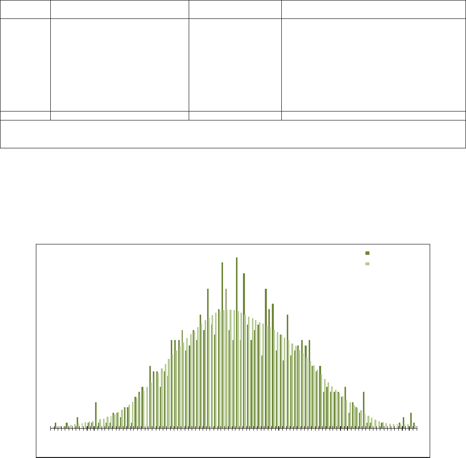
Casualty Actuarial Society 85
Using the ODP Bootstrap Model: A Practitioner’s Guide
Five Top 50 Companies
Schedule P, Part B -- Private Passenger Auto Liability (in 000,000’s)
Accident Year Unpaid
Incurred GLM Bootstrap Model
Accident Mean Standard Coefficient50.0% 75.0%95.0% 99.0%
Year Unpaid Error of Variation MinimumMaximum Percentile Percentile Percentile Percentile
2006 28 15 55.2% 3110 25 35 58 76
2007 56 24 42.7% 7178 53 69 10
21
38
2008 107 33 30.8% 43 298101 127168 200
2009 172 34 19.6% 91 301169 191235 263
2010 295 36 12.4% 204 419290 316361 394
2011 568 49 8.6% 434 764565 597652 702
2012 1,130 90 8.0% 857 1,4221,126 1,1891,285 1,332
2013 2,193 168 7.7% 1,738 2,8842,193 2,3072,468 2,605
2014 4,058 319 7.9% 3,096 5,0404,063 4,2944,573 4,764
2015 8,390 723 8.6% 5,922 10,670 8,3758,917 9,52
49
,986
Totals 16,996 985 5.8% 13,965 19,871 16,965 17,696 18,619 19,079
Normal Dist. 16,996 985 5.8% 16,996 17,660 18,616 19,287
logNormal Dist. 16,996 989 5.8% 16,967 17,645 18,669 19,424
Gamma Dist. 16,996 985 5.8% 16,977 17,649 18,647 19,371
Figure B.15. Estimated Unpaid Model Results (Incurred GLM)
Five Top 50 Companies
Schedule P, Part B -- Private Passenger Auto Liability (in 000,000’s)
Total Unpaid Distribution
Incurred GLM Bootstrap Model
13.9K 14.5K 15.1K 15.7K 16.3K 16.9K 17.5K 18.1K 18.7K 19.3K 19.9K
Probability
Total Unpaid
Histogram
Kernel Density
Figure B.16. Total Unpaid Claims Distribution (Incurred GLM)

86 Casualty Actuarial Society
Using the ODP Bootstrap Model: A Practitioner’s Guide
AccidentModel Weights by Accident Year
Year Paid CL Incd CL Paid BF Incd BF Paid CC Incd CC Paid GLM Incd GLM TOTAL
2006 50.0% 50.0% 100.0%
2007 50.0% 50.0% 100.0%
2008 50.0% 50.0% 100.0%
2009 50.0% 50.0% 100.0%
2010 25.0%25.0% 25.0%25.0% 100.0%
2011 25.0%25.0% 25.0%25.0% 100.0%
2012 25.0%25.0% 25.0%25.0% 100.0%
2013 25.0%25.0% 25.0%25.0% 100.0%
2014 25.0%25.0% 25.0% 25.0% 100.0%
2015 25.0%25.0% 25.0% 25.0% 100.0%
Figure B.17. Model Weights by Accident Year
Five Top 50 Companies
Schedule P, Part B -- Private Passenger Auto Liability (in 000,000’s)
Summary of Results by Model
Mean Estimated Unpaid
Accident Chain Ladder Bornhuetter-Ferguson Cape CodGLM Bootstrap Best Est.
Year Paid Incurred Paid Incurred PaidIncurred PaidIncurred (Weighted)
2006 59 58 54 54 55 56 29 28 59
2007 90 89 76 76 80 80 56 56 90
2008 135135 112 111 117 118 99 107 134
2009 214213 188 188 196 197 177 172 214
2010 339343 343 344 354 358 302 295 351
2011 586590 625 627 642 650 552 568 636
2012 1,109 1,125 1,162 1,167 1,197 1,201 1,071 1,130 1,184
2013 2,089 2,133 2,217 2,234 2,292 2,308 2,053 2,193 2,255
2014 3,917 4,025 3,942 3,997 4,145 4,178 3,879 4,058 4,077
2015 8,033 8,343 7,990 8,289 8,598 8,526 8,004 8,390 8,394
Totals 16,573 17,054 16,709 17,088 17,676 17,672 16,222 16,996 17,395
Figure B.18. Estimated Mean Unpaid by Model
Five Top 50 Companies
Schedule P, Part B -- Private Passenger Auto Liability (in 000,000’s)
Summary of Results by Model
Ranges
Accident Best Est. Weighted Modeled
Year (Weighted) Minimum Maximum Mininum Maximum
2006 59 58 59 28 59
2007 90 89 90 56 90
2008 134 135 135 107 135
2009 214 213 214 172 214
2010 351 343 358 295 358
2011 636 625 650 568 650
2012 1,184 1,162 1,201 1,109 1,201
2013 2,255 2,217 2,308 2,089 2,308
2014 4,077 3,997 4,178 3,917 4,178
2015 8,394 8,289 8,526 7,990 8,598
Totals 17,395 17,127 17,720 16,573 17,676
Figure B.19. Estimated Ranges

Casualty Actuarial Society 87
Using the ODP Bootstrap Model: A Practitioner’s Guide
Five Top 50 Companies
Schedule P, Part B -- Private Passenger Auto Liability (in 000,000’s)
Reconciliation of Total Results
Best Estimate (Weighted)
Accident Paid Incurred Case Estimate of Estimate of
Year To Date To Date Reserves IBNR Ultimate Unpaid
2006 11,816 11,863 47 12 11,875 59
2007 12,679 12,752 72 18 12,770 90
2008 13,631 13,743 1122213,76
51
34
2009 14,472 14,687 216 (1) 14,686 214
2010 13,717 14,079 362 (11) 14,068 351
2011 13,090 13,691 6003613,72
66
36
2012 12,490 13,683 1,193 (9) 13,674 1,184
2013 11,598 13,912 2,313 (58) 13,854 2,255
2014 10,306 14,625 4,319 (243)14,383 4,077
2015 6,357 15,188 8,830 (437)14,751 8,394
Totals 120,157 138,223 18,066 (671)137,551 17,395
Figure B.20. Reconciliation of Total Results (Weighted)
Five Top 50 Companies
Schedule P, Part B -- Private Passenger Auto Liability (in 000,000’s)
Accident Year Unpaid
Best Estimate (Weighted)
Accident Mean Standard Coefficient 50.0%75.0% 95.0%99.0%
Year UnpaidError of VariationMinimum Maximum Percentile Percentile Percentile Percentile
2006 59 25 42.2% -178 58 75 10
21
22
2007 90 28 30.8% 17 22189109 13
71
61
2008 134 32 24.0% 41 297133 156189 215
2009 214 41 18.9% 73 401213 240284 321
2010 351 55 15.6% 160 600350 383444 492
2011 636 91 14.2% 314 1,020636 684794 867
2012 1,184 157 13.3% (27) 1,8571,188 1,2601,465 1,597
2013 2,255 293 13.0% 1,073 5,7102,267 2,3892,781 2,982
2014 4,077 616 15.1% 833 6,0494,097 4,4605,120 5,398
2015 8,394 1,234 14.7% 980 12,352 8,4689,175 10,444 10,911
Totals 17,395 1,428 8.2% 10,057 23,150 17,439 18,375 19,729 20,525
Normal Dist. 17,395 1,428 8.2% 17,395 18,358 19,744 20,717
logNormal Dist. 17,395 1,451 8.3% 17,335 18,336 19,879 21,040
Gamma Dist. 17,395 1,428 8.2% 17,356 18,336 19,809 20,889
Figure B.21. Estimated Unpaid Model Results (Weighted)

88 Casualty Actuarial Society
Using the ODP Bootstrap Model: A Practitioner’s Guide
Five Top 50 Companies
Schedule P, Part B -- Private Passenger Auto Liability (in 000,000’s)
Calendar Year Unpaid
Best Estimate (Weighted)
Calendar Mean Standard Coefficient 50.0%75.0% 95.0%99.0%
Year Unpaid Error of Variation Minimum Maximum Percentile Percentile Percentile Percentile
2016 8,275 715 8.6% 4,501 10,746 8,2998,761 9,42
69
,838
2017 4,072 340 8.4% 2,450 5,6084,079 4,3044,621 4,845
2018 2,266 198 8.7% 1,319 3,1492,267 2,3972,590 2,718
2019 1,210 109 9.0% 699 1,5741,210 1,2851,389 1,461
2020 638 58 9.1% 405 885638 677735 778
2021 358 35 9.8% 203 511358 381416 439
2022 217 30 13.7% 95 351216 237267 291
2023 144 25 17.2% 57 258144 161186 205
2024 99 23 23.4% 16 21498114 13
91
57
2025 67 22 33.1% -157 66 81 10
61
24
2026 32 13 40.8% -9132415
56
6
2027 16 9 57.3% -5715223
13
8
Totals 17,395 1,428 8.2% 10,057 23,150 17,439 18,375 19,729 20,525
Figure B.22. Estimated Cash Flow (Weighted)
Five Top 50 Companies
Schedule P, Part B -- Private Passenger Auto Liability (in 000,000’s)
Accident Year Ultimate Loss Ratios
Best Estimate (Weighted)
Accident Mean Standard Coefficient 50.0%75.0% 95.0%99.0%
Year Loss RatioError of Variation Minimum Maximum Percentile Percentile Percentile Percentile
2006 75.6% 9.7% 12.9% 38.9% 104.5% 75.8%77.8% 94.6
%9
9.4%
2007 82.2% 10.3% 12.5% 43.9% 114.0% 82.4%84.6% 102.2% 107.6%
2008 83.9% 10.2% 12.1% 45.1% 114.4% 83.9%86.3% 103.7% 108.6%
2009 79.6% 9.2% 11.6% 45.2% 108.3% 79.7%81.8% 97.8
%1
02.7%
2010 69.3% 8.2% 11.9% 37.9% 94.6%69.1% 71.1%85.3% 90.1%
2011 66.0% 8.1% 12.3% 35.2% 89.7%66.0% 67.9%81.7% 85.9%
2012 66.9% 8.1% 12.1% -1.5% 94.6%66.9% 68.8%82.7% 86.8%
2013 66.9% 8.1% 12.2% 35.2% 186.1% 66.9%68.9% 82.4
%8
6.3%
2014 71.9% 10.6% 14.7% 14.4% 101.9% 72.7%78.5% 89.0
%9
3.5%
2015 73.0% 10.6% 14.5% 8.4% 110.0% 73.9%79.8% 90.3
%9
4.2%
Totals 72.9% 3.0% 4.1% 61.6% 90.9%73.0% 75.0%77.7% 79.5%
Figure B.23. Estimated Loss Ratio (Weighted)
Five Top 50 Companies
Schedule P, Part B -- Private Passenger Auto Liability (in 000,000’s)
Calendar Year Unpaid Claim Runoff
Best Estimate (Weighted)
Calendar Mean Standard Coefficient 50.0%75.0% 95.0%99.0%
Year Unpaid Error of Variation Minimum Maximum Percentile Percentile Percentile Percentile
2015 17,395 1,428 8.2% 10,057 23,150 17,439 18,375 19,729 20,525
2016 9,120 739 8.1% 5,556 12,446 9,1369,623 10,325 10,767
2017 5,048 419 8.3% 3,106 6,8385,054 5,3305,738 6,000
2018 2,782 243 8.7% 1,709 3,6892,781 2,9453,184 3,360
2019 1,572 157 10.0% 902 2,1651,570 1,6751,838 1,951
2020 934 117 12.6% 494 1,387930 1,0111,131 1,224
2021 576 94 16.3% 247 988573 638733 807
2022 359 75 21.0% 104 687356 408488 546
2023 214 59 27.6% 30 467211 252317 365
2024 115 41 36.0% (0) 283112 142188 222
2025 48 20 42.4% (0) 13747628
41
01
2026 16 9 57.3% (0) 57 15 22 31 38
2027 (0) 0 -10502.4% (0) 0(0) 000
Figure B.24. Estimated Unpaid Claim Runoff (Weighted)
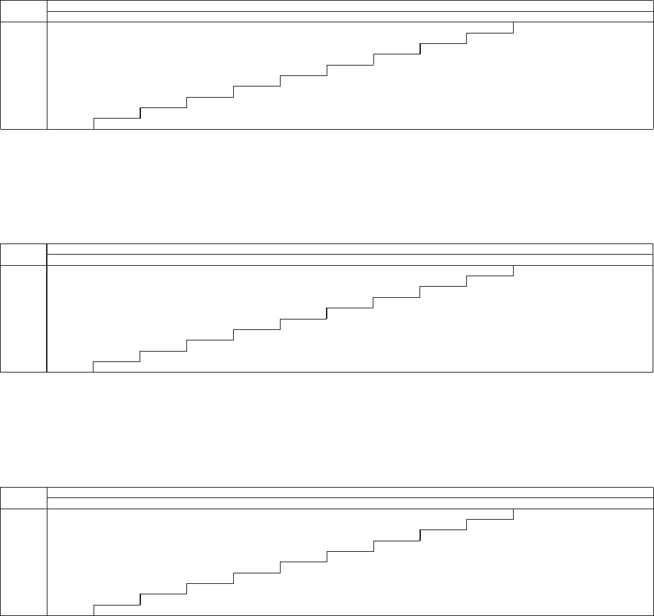
Casualty Actuarial Society 89
Using the ODP Bootstrap Model: A Practitioner’s Guide
Five Top 50 Companies
Schedule P, Part B -- Private Passenger Auto Liability (in 000,000’s)
Accident Year Incremental Values by Development Period
Best Estimate (Weighted)
Accident Mean Values
Year 12 24 36 48 60 72 84 96 108 120 132 144 156 +
2006 5,232 3,354 1,456 842 457 224 113 58 32 25 30 15 15
2007 5,631 3,608 1,566 907 491 241 121 62 34 27 32 16 16
2008 6,082 3,902 1,691 981 530 261 131 67 37 29 34 17 17
2009 6,480 4,155 1,802 1,043 565 278 139 71 39 31 36 18 18
2010 6,225 3,992 1,732 1,002 543 267 138 71 39 31 36 18 18
2011 6,043 3,876 1,681 974 527 280 141 72 40 31 36 18 18
2012 6,008 3,851 1,671 968 560 274 138 71 39 31 36 18 18
2013 6,046 3,876 1,681 1,051 569 279 140 72 40 31 36 18 18
2014 6,453 4,138 1,821 1,055 572 281 141 72 41 30 32 17 16
2015 6,549 4,261 1,847 1,070 579 284 143 73 41 31 32 17 16
Figure B.25. Mean of Incremental Values (Weighted)
Five Top 50 Companies
Schedule P, Part B -- Private Passenger Auto Liability (in 000,000’s)
Accident Year Incremental Values by Development Period
Best Estimate (Weighted)
Accident Standard Error Values
Year 12 24 36 48 60 72 84 96 108 120 132 144 156 +
2006 677 440 199 115 65 35 15 12 4312
66
2007 708 460 207 120 68 36 16 13 4313
77
2008 742 484 217 126 70 38 16 13 5414
77
2009 756 493 220 129 72 39 17 16 5415
88
2010 745 485 218 127 71 38 18 16 5415
88
2011 747 486 218 128 71 44 19 16 5415
88
2012 729 475 213 124 78 42 18 16 5415
88
2013 741 483 218 142 79 43 19 16 5415
88
2014 955 618 282 165 92 47 22 18 8717
99
2015 966 634 280 166 92 48 22 18 9717
99
Figure B.26. Standard Deviation of Incremental Values (Weighted)
Five Top 50 Companies
Schedule P, Part B -- Private Passenger Auto Liability (in 000,000’s)
Accident Year Incremental Values by Development Period
Best Estimate (Weighted)
Accident Coefficients of Variation
Year 12 24 36 48 60 72 84 96 108 120 132 144 156 +
2006 12.9% 13.1% 13.6% 13.7% 14.2% 15.5% 13.4% 21.2% 12.9% 12.9% 42.1% 42.2% 42.3%
2007 12.6% 12.7% 13.2% 13.3% 13.8% 15.0% 13.0% 20.6% 12.5% 12.6% 42.0% 42.1% 42.2%
2008 12.2% 12.4% 12.8% 12.8% 13.3% 14.5% 12.6% 19.9% 12.2% 12.3% 42.3% 42.4% 42.5%
2009 11.7% 11.9% 12.2% 12.4% 12.7% 13.9% 12.1% 22.0% 11.7% 11.7% 42.0% 42.1% 42.2%
2010 12.0% 12.2% 12.6% 12.6% 13.1% 14.3% 13.1% 22.5% 12.5% 12.6% 42.5% 42.6% 42.7%
2011 12.4% 12.5% 13.0% 13.1% 13.5% 15.6% 13.4% 22.5% 12.9% 12.9% 42.5% 42.7% 42.8%
2012 12.1% 12.3% 12.8% 12.9% 13.9% 15.3% 13.2% 22.4% 12.6% 12.7% 42.3% 42.5% 42.5%
2013 12.3% 12.5% 13.0% 13.5% 13.9% 15.4% 13.2% 22.3% 12.7% 12.7% 42.0% 42.2% 42.2%
2014 14.8% 14.9% 15.5% 15.7% 16.1% 16.8% 15.4% 24.5% 20.8% 23.7% 52.6% 51.2% 57.5%
2015 14.7% 14.9% 15.2% 15.5% 15.9% 16.7% 15.2% 24.4% 20.6% 23.4% 52.1% 51.1% 57.3%
Figure B.27. Coefficient of Variation of Incremental Values (Weighted)
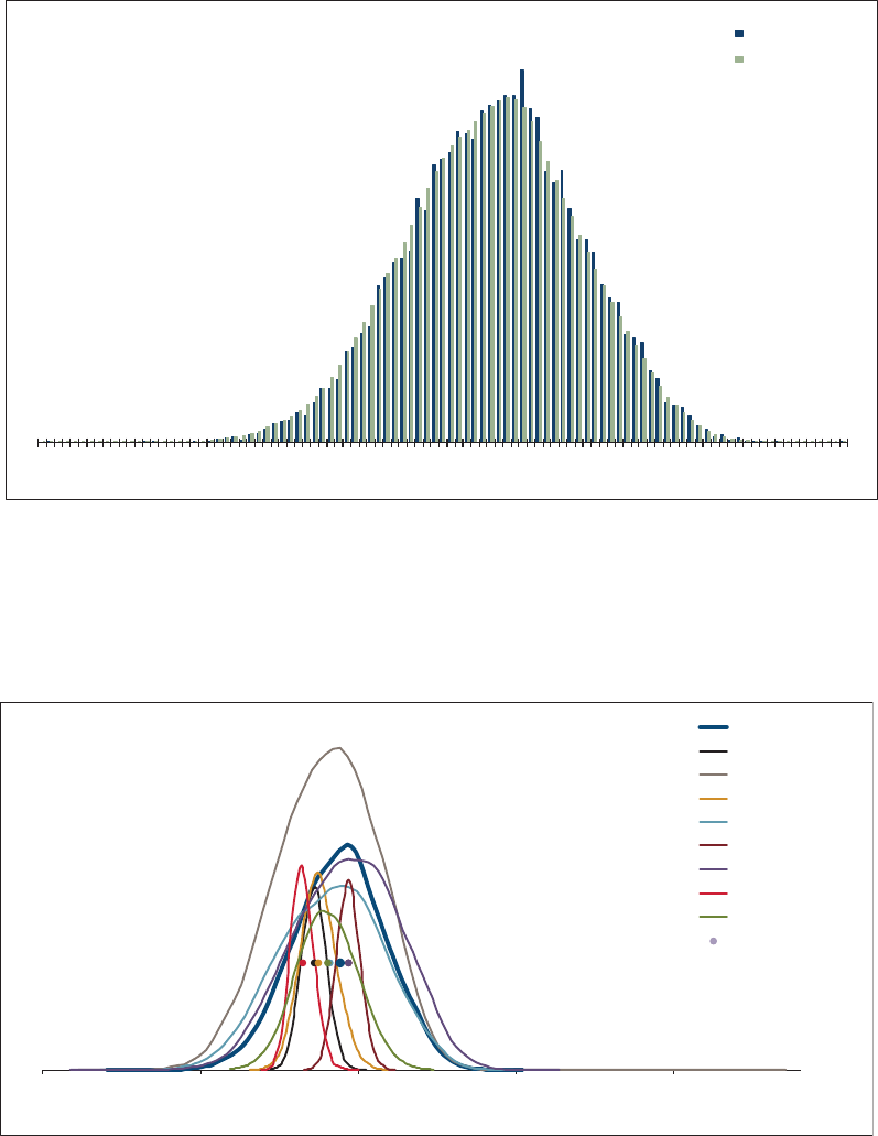
90 Casualty Actuarial Society
Using the ODP Bootstrap Model: A Practitioner’s Guide
Five Top 50 Companies
Schedule P, Part B -- Private Passenger Auto Liability (in 000,000’s)
Total Unpaid Distribution
Best Estimate (Weighted)
10.0K11.3K 12.6K14.0K 15.3K16.6K 17.9K 19.2K20.6K 21.9K 23.2K
Probability
Total Unpaid
Histogram
Kernel Density
Figure B.28. Total Unpaid Claims Distribution (Weighted)
Five Top 50 Companies
Schedule P, Part B -- Private Passenger Auto Liability (in 000,000’s)
Summary of Model Distributions
(Using Kernel Densities)
8.0K 13.0K 18.0K 23.0K 28.0K
Probability
Total Unpaid
Best Estimate
Paid CL
Incurred CL
Paid BF
Incurred BF
Paid CC
Incurred CC
Paid GLM
Incurred GLM
Mean Estimates
Figure B.29. Summary of Model Distributions
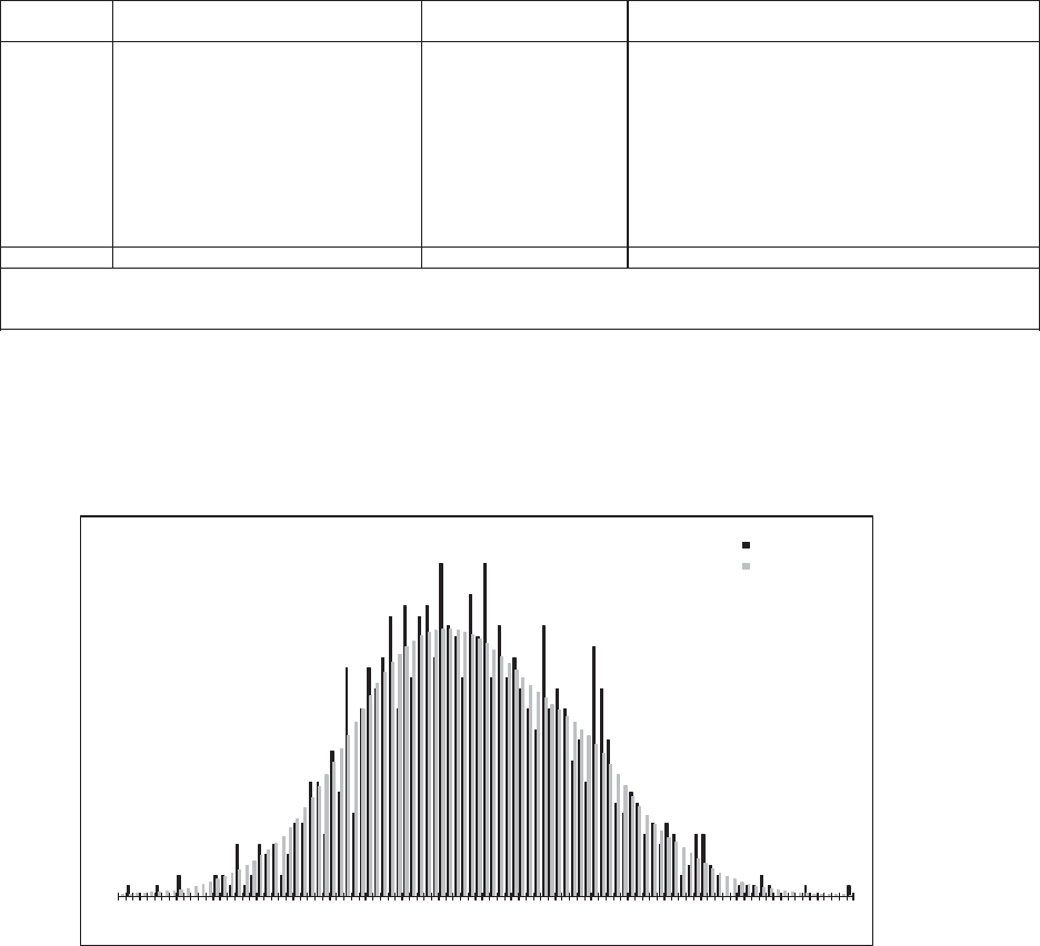
Casualty Actuarial Society 91
Appendix C—Schedule P, Part C Results
In this appendix the results for Schedule P, Part C (Commercial Auto Liability) are shown.
Five Top 50 Companies
Schedule P, Part C – Commercial Auto Liability (in 000,000's)
Accident Year Unpaid
Paid Chain Ladder Model
Accident Mean Standard Coefficient50.0% 75.0%95.0% 99.0%
YearUnpaid Error of Variation MinimumMaximum Percentile Percentile Percentile Percentile
2006 8450.6% -22810 15 19
2007 11 4 39.9% (0) 28 10 13 18 22
2008 21 5 24.3% 74321242
93
4
2009 35 6 18.3% 18 66 34 39 46 51
2010 61 10 16.6% 34 97 60 67 80 87
2011 110 22 20.0% 57 195107 124150 173
2012 216 33 15.4% 111 359215 237273 296
2013 410 39 9.4% 294 550408 434474 513
2014 773 52 6.7% 610 946770 806863 901
2015 1,103 75 6.8% 872 1,3451,100 1,1521,232 1,285
Totals 2,746 122 4.4% 2,357 3,1712,741 2,8302,951 3,019
Normal Dist. 2,746 122 4.4% 2,7462,828 2,94
63
,029
logNormal Dist. 2,746 122 4.4% 2,7432,827 2,95
13
,041
Gamma Dist. 2,746 122 4.4% 2,7442,827 2,94
93
,037
Figure C.1. Estimated Unpaid Model Results (Paid Chain Ladder)
Five Top 50 Companies
Schedule P, Part C – Commercial Auto Liability (in 000,000's)
Total Unpaid Distribution
Paid Chain Ladder Model
2.35K 2.43K 2.52K 2.60K 2.68K 2.76K 2.85K 2.93K 3.01K 3.09K 3.18K
Probability
Total Unpaid
Histogram
Kernel Density
Figure C.2. Total Unpaid Claims Distribution (Paid Chain Ladder)
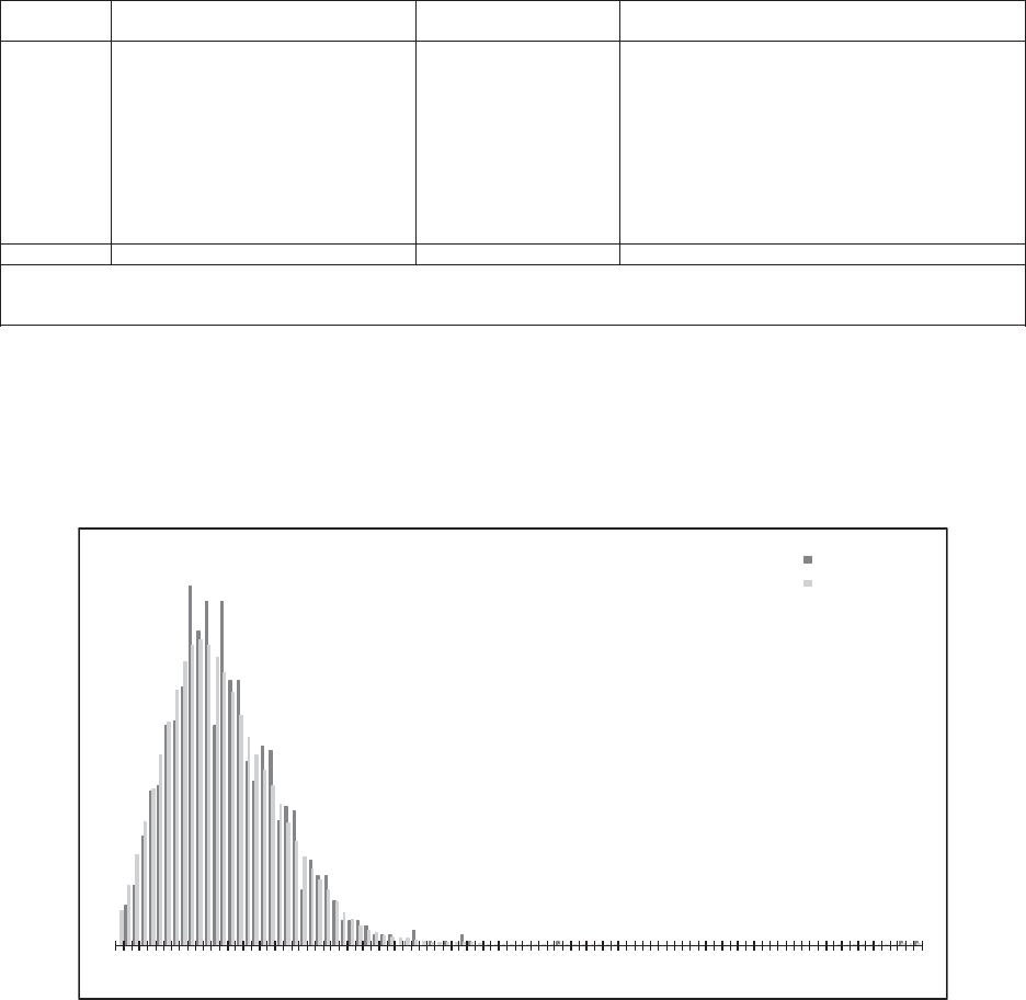
92 Casualty Actuarial Society
Using the ODP Bootstrap Model: A Practitioner’s Guide
Five Top 50 Companies
Schedule P, Part C -- Commercial Auto Liability (in 000,000's)
Accident Year Unpaid
Incurred Chain Ladder Model
Accident Mean Standard Coefficient50.0% 75.0%95.0% 99.0%
Year Unpaid Error of Variation Minimum MaximumPercentile Percentile Percentile Percentile
2006 11 12 108.0% -74716 35 48
2007 15 16 110.1% 0157 9224
66
6
2008 31 33 105.0% -354 23 47 91 127
2009 53 54 102.3% -533 41 86 14
42
00
2010 92 103 111.1% -1,654 69 145258 369
2011 168 176 104.5% -1,625 127264 49
86
81
2012 328 372 113.3% -4,031 217528 96
31
,307
2013 623 615 98.7% -3,767 4841,049 1,78
22
,238
2014 1,223 1,415 115.7% -21,8021,019 2,0103,319 4,335
2015 1,513 1,618 107.0% -13,8301,062 2,5464,356 5,798
Totals 4,056 2,421 59.7% 146 30,092 3,7255,273 7,78
61
0,983
Normal Dist. 4,056 2,421 59.7% 4,0565,689 8,03
89
,687
logNormal Dist. 4,168 2,899 69.6% 3,4225,227 9,61
61
4,755
Gamma Dist. 4,056 2,421 59.7% 3,5865,328 8,67
71
1,670
Figure C.3. Estimated Unpaid Model Results (Incurred Chain Ladder)
Five Top 50 Companies
Schedule P, Part C – Commercial Auto Liability (in 000,000's)
Total Unpaid Distribution
Incurred Chain Ladder Model
1.00 3.1K 6.1K 9.1K 12.1K 15.1K 18.1K 21.1K 24.1K 27.1K 30.1K
Probability
Total Unpaid
Histogram
Kernel Density
Figure C.4. Total Unpaid Claims Distribution (Incurred Chain Ladder)
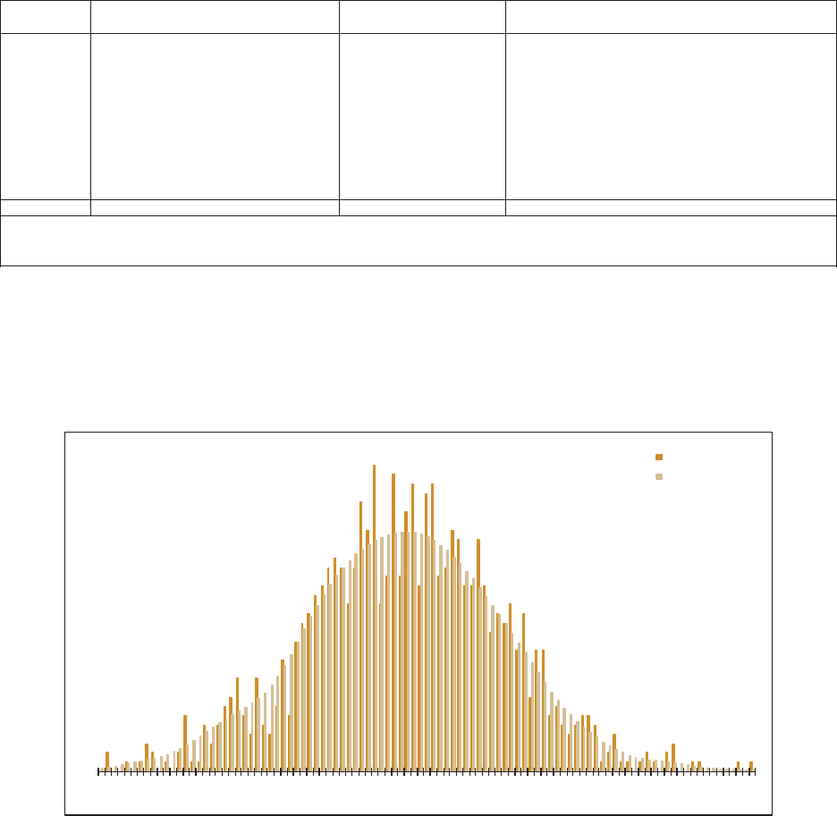
Casualty Actuarial Society 93
Using the ODP Bootstrap Model: A Practitioner’s Guide
Five Top 50 Companies
Schedule P, Part C -- Commercial Auto Liability (in 000,000's)
Accident Year Unpaid
Paid Bornhuetter-Ferguson Model
Accident Mean Standard Coefficient50.0% 75.0%95.0% 99.0%
Year Unpaid Error of Variation MinimumMaximum Percentile Percentile Percentile Percentile
2006 5354.4% -16571
01
3
2007 8342.3% 022810 14 17
2008 17 4 26.7% 53217202
52
9
2009 35 7 19.3% 13 64 34 39 46 52
2010 65 11 17.1% 38 11065738
49
4
2011 123 25 20.5% 44 211121 140167 197
2012 259 40 15.6% 145 420256 287327 353
2013 481 52 10.8% 315 658477 517565 607
2014 812 76 9.3% 590 1,078811 860936 996
2015 1,132 100 8.9% 857 1,4801,127 1,1981,300 1,369
Totals 2,936 153 5.2% 2,472 3,4742,939 3,0403,180 3,313
Normal Dist. 2,936 153 5.2% 2,9363,040 3,18
83
,293
logNormal Dist. 2,936 154 5.2% 2,9323,038 3,19
63
,312
Gamma Dist. 2,936 153 5.2% 2,9343,038 3,19
33
,305
Figure C.5. Estimated Unpaid Model Results (Paid Bornhuetter-Ferguson)
Five Top 50 Companies
Schedule P, Part C -- Commercial Auto Liability (in 000,000's)
Total Unpaid Distribution
Paid Bornhuetter-Ferguson Model
2.5K 2.6K 2.7K 2.8K 2.9K 3.0K 3.1K 3.2K 3.3K 3.4K 3.5K
Probability
Total Unpaid
Histogram
Kernel Density
Figure C.6. Total Unpaid Claims Distribution (Paid Bornhuetter-Ferguson)
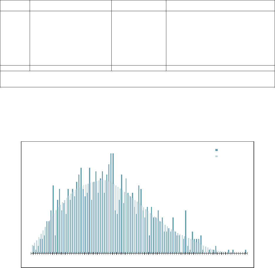
94 Casualty Actuarial Society
Using the ODP Bootstrap Model: A Practitioner’s Guide
Five Top 50 Companies
Schedule P, Part C – Commercial Auto Liability (in 000,000's)
Accident Year Unpaid
Incurred Bornhuetter-Ferguson Model
Accident Mean Standard Coefficient50.0% 75.0%95.0% 99.0%
YearUnpaid Error of Variation MinimumMaximum Percentile Percentile Percentile Percentile
2006 78116.0% -48410 24 34
2007 11 12 110.5% -61715 36 52
2008 24 23 96.0% -124 18 37 68 93
2009 49 45 92.9% -216 38 80 13
91
65
2010 99 88 88.8% 0375 82 162265 318
2011 176 164 93.3% 0821 134279 50
56
30
2012 362 338 93.5% 01,547 296584 1,00
51
,228
2013 642 597 93.1% 12,344 5021,066 1,79
22
,119
2014 1,118 996 89.1% 04,243 9801,862 2,91
93
,447
2015 1,554 1,409 90.6% 05,956 1,3712,626 4,14
64
,729
Totals 4,040 1,873 46.4% 387 10,575 3,9015,304 7,41
88
,445
Normal Dist. 4,040 1,873 46.4% 4,0405,303 7,12
08
,397
logNormal Dist. 4,116 2,390 58.1% 3,5605,120 8,63
81
2,472
Gamma Dist. 4,040 1,873 46.4% 3,7555,099 7,53
09
,612
Figure C.7. Estimated Unpaid Model Results (Incurred Bornhuetter-Ferguson)
Five Top 50 Companies
Schedule P, Part C -- Commercial Auto Liability (in 000,000's)
Total Unpaid Distribution
Incurred Bornhuetter-Ferguson Model
340 1.4K 2.4K 3.4K 4.5K 5.5K 6.5K 7.5K 8.6K 9.6K 10.6K
Probability
Total Unpaid
Histogram
Kernel Density
Figure C.8. Total Unpaid Claims Distribution (Incurred Bornhuetter-Ferguson)
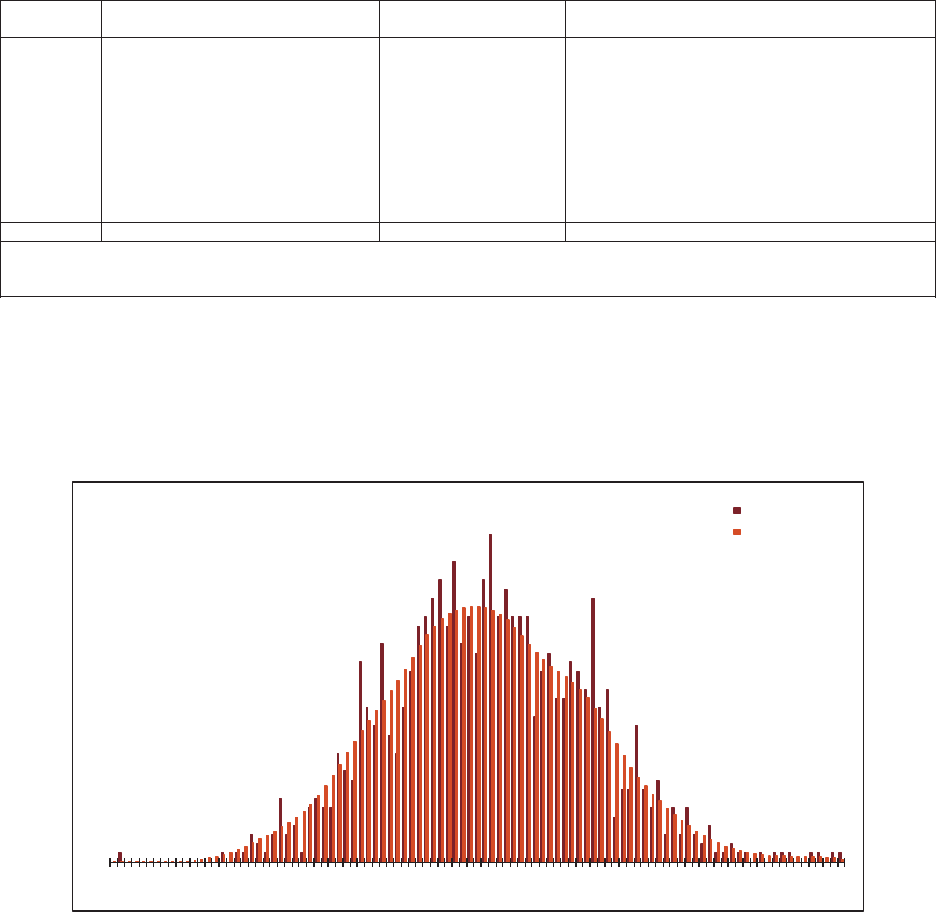
Casualty Actuarial Society 95
Using the ODP Bootstrap Model: A Practitioner’s Guide
Five Top 50 Companies
Schedule P, Part C – Commercial Auto Liability (in 000,000's)
Accident Year Unpaid
Paid Cape Cod Model
Accident Mean Standard Coefficient50.0% 75.0%95.0% 99.0%
YearUnpaid Error of Variation MinimumMaximum Percentile Percentile Percentile Percentile
2006 6352.3% -17681
21
4
2007 9441.0% 026911 15 19
2008 18 5 26.1% 73418222
73
1
2009 36 7 17.9% 20 59 36 41 48 52
2010 67 11 16.1% 39 10166748
69
4
2011 124 23 18.8% 67 245122 138163 192
2012 258 38 14.8% 166 416255 283323 359
2013 481 40 8.4% 363 629478 509548 583
2014 827 50 6.0% 684 975827 858915 948
2015 1,178 53 4.5% 990 1,3481,176 1,2121,268 1,308
Totals 3,004 122 4.0% 2,559 3,4283,001 3,0883,204 3,297
Normal Dist. 3,004 122 4.0% 3,0043,086 3,20
43
,286
logNormal Dist. 3,004 121 4.0% 3,0013,084 3,20
83
,297
Gamma Dist. 3,004 122 4.0% 3,0023,085 3,20
63
,294
Figure C.9. Estimated Unpaid Model Results (Paid Cape Cod)
Five Top 50 Companies
Schedule P, Part C -- Commercial Auto Liability (in 000,000's)
Total Unpaid Distribution
Paid Cape Cod Model
2.6K 2.6K 2.7K 2.8K 2.9K 3.0K 3.1K 3.2K 3.3K 3.3K 3.4K
Probability
Total Unpaid
Histogram
Kernel Density
Figure C.10. Total Unpaid Claims Distribution (Paid Cape Cod)
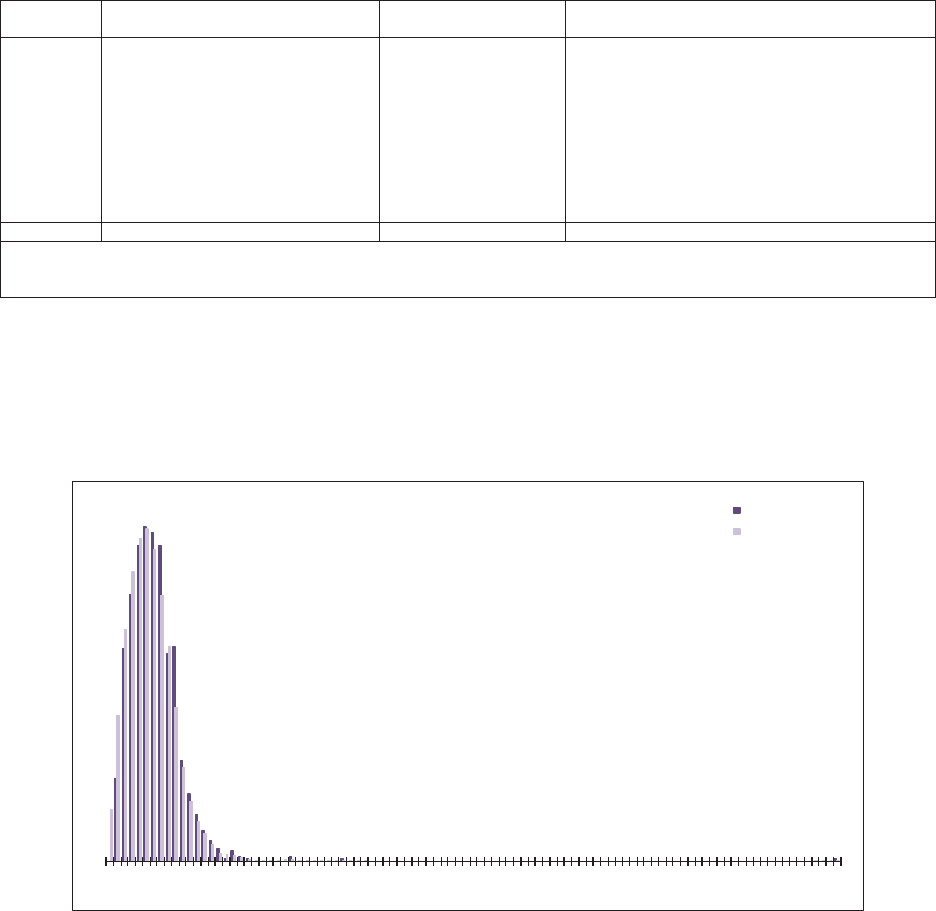
96 Casualty Actuarial Society
Using the ODP Bootstrap Model: A Practitioner’s Guide
Five Top 50 Companies
Schedule P, Part C -- Commercial Auto Liability (in 000,000's)
Accident Year Unpaid
Incurred Cape Cod Model
Accident Mean Standard Coefficient50.0% 75.0%95.0% 99.0%
Year Unpaid Error of Variation MinimumMaximum Percentile Percentile Percentile Percentile
2006 89110.7% -62512 25 36
2007 13 14 108.2% -98919 43 60
2008 25 25 98.6% 0185 18 40 76 99
2009 52 51 98.2% 0481 37 82 14
52
01
2010 101 98 97.9% 01,082 81 160267 339
2011 183 199 108.7% 03,031 140282 51
56
44
2012 403 410 101.7% 04,350 320637 1,10
61
,514
2013 696 747 107.4% 011,739577 1,1101,930 2,405
2014 1,287 1,239 96.3% 020,3221,121 2,0453,306 4,162
2015 1,647 1,748 106.1% 131,0781,408 2,6944,317 5,401
Totals 4,415 3,174 71.9% 372 72,036 4,0895,685 8,35
71
1,920
Normal Dist. 4,415 3,174 71.9% 4,4156,555 9,63
51
1,797
logNormal Dist. 4,465 2,906 65.1% 3,7435,588 9,94
71
4,914
Gamma Dist. 4,415 3,174 71.9% 3,6825,956 10,581 14,867
Figure C.11. Estimated Unpaid Model Results (Incurred Cape Cod)
Five Top 50 Companies
Schedule P, Part C – Commercial Auto Liability (in 000,000's)
Total Unpaid Distribution
Incurred Cape Cod Model
320 7.5K 14.7K 21.9K 29.0K 36.2K 43.4K50.6K 57.7K 64.9K 72.1K
Probability
Total Unpaid
Histogram
Kernel Density
Figure C.12. Total Unpaid Claims Distribution (Incurred Cape Cod)
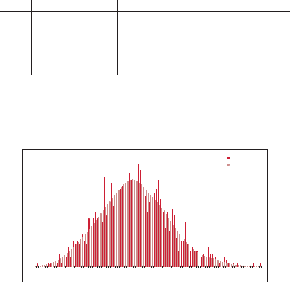
Casualty Actuarial Society 97
Using the ODP Bootstrap Model: A Practitioner’s Guide
Five Top 50 Companies
Schedule P, Part C – Commercial Auto Liability (in 000,000's)
Accident Year Unpaid
Paid GLM Bootstrap Model
Accident Mean StandardCoefficient 50.0% 75.0% 95.0% 99.0%
Year Unpaid Error of Variation Minimum MaximumPercentile Percentile Percentile Percentile
2006 8563.7% (5) 33 7101
72
3
2007 14 7 52.9% (3) 52 12 18 27 33
2008 23 9 39.9% (1) 72 22 29 39 49
2009 38 12 30.2% 89038455
87
0
2010 64 13 20.8% 27 112 64 73 88 100
2011 123 17 13.8% 81 178 122 135 152 162
2012 244 25 10.4% 169 331 243 261 286 305
2013 457 37 8.1% 361 577 455 480 520 543
2014 747 53 7.1% 597 926 749 784 831 870
2015 1,063 77 7.3% 851 1,346 1,060 1,112 1,192 1,259
Totals 2,781 188 6.8% 2,234 3,480 2,775 2,904 3,097 3,251
Normal Dist. 2,781 188 6.8% 2,781 2,907 3,090 3,218
logNormal Dist. 2,781 188 6.8% 2,774 2,903 3,100 3,246
Gamma Dist. 2,781 188 6.8% 2,776 2,905 3,097 3,237
Figure C.13. Estimated Unpaid Model Results (Paid GLM)
Five Top 50 Companies
Schedule P, Part C – Commercial Auto Liability (in 000,000's)
Total Unpaid Distribution
Paid GLM Bootstrap Model
2.2K 2.4K 2.5K 2.6K 2.7K 2.9K3.0K3.1K3.2K3.4
K3
.5K
Probability
Total Unpaid
Histogram
Kernel Density
Figure C.14. Total Unpaid Claims Distribution (Paid GLM)
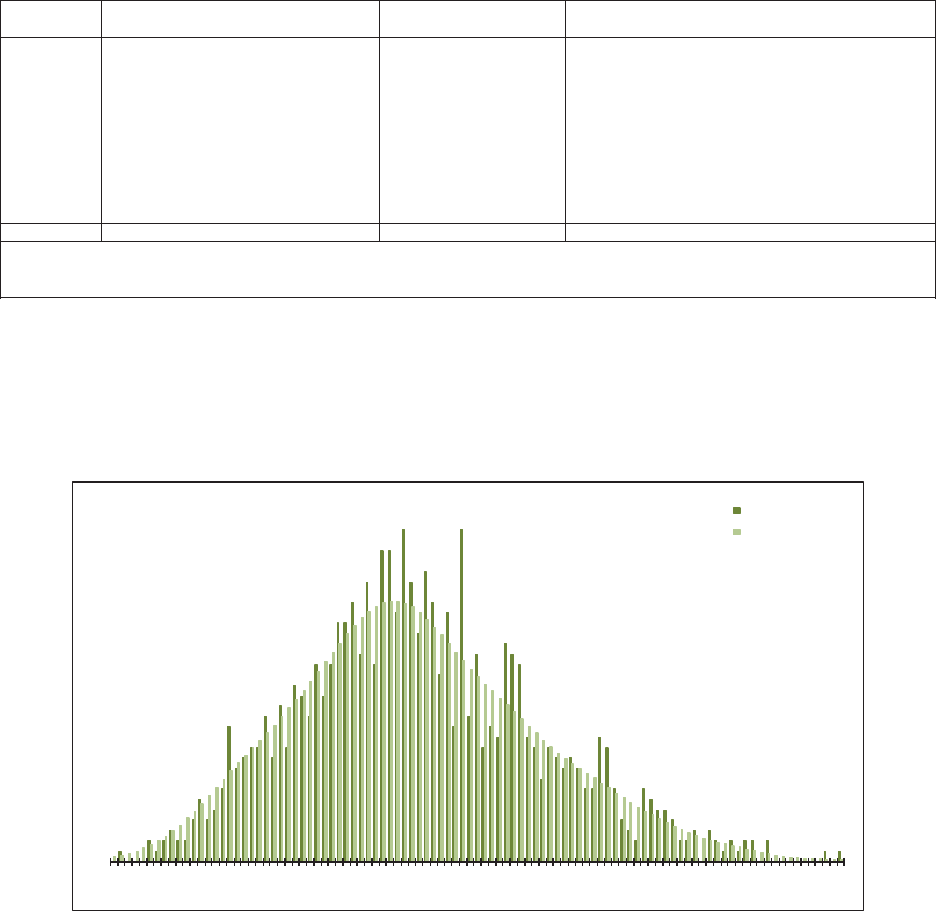
98 Casualty Actuarial Society
Using the ODP Bootstrap Model: A Practitioner’s Guide
Five Top 50 Companies
Schedule P, Part C – Commercial Auto Liability (in 000,000's)
Accident Year Unpaid
Incurred GLM Bootstrap Model
AccidentMean Standard Coefficient 50.0%75.0% 95.0%99.0%
Year Unpaid Error of Variation MinimumMaximum Percentile Percentile Percentile Percentile
2006 10 8 81.9% (9) 57 8132
53
9
2007 17 11 62.4% (5) 65 15 22 39 53
2008 31 17 53.2% (0) 10429406
38
2
2009 54 23 43.3% 7177 50 67 97 119
2010 92 35 38.2% 17 25188113 15
31
84
2011 174 63 36.1% 23 378171 217278 333
2012 363 119 32.8% 76 773360 443572 648
2013 682 224 32.9% 100 1,490666 8331,078 1,211
2014 1,097 366 33.3% 267 2,3461,084 1,3341,716 2,055
2015 1,567 555 35.4% 452 4,0271,515 1,8992,536 3,071
Totals 4,087 760 18.6% 2,190 6,7544,018 4,5845,485 6,034
Normal Dist. 4,087 760 18.6% 4,0874,599 5,33
65
,854
logNormal Dist. 4,087 769 18.8% 4,0174,555 5,46
06
,200
Gamma Dist. 4,087 760 18.6% 4,0404,570 5,41
16
,058
Figure C.15. Estimated Unpaid Model Results (Incurred GLM)
Five Top 50 Companies
Schedule P, Part C – Commercial Auto Liability (in 000,000's)
Total Unpaid Distribution
Incurred GLM Bootstrap Model
2.2K 2.6K 3.1K 3.6K 4.0K 4.5K4.9K5.4K5.8K6.3
K6
.8K
Probability
Total Unpaid
Histogram
Kernel Density
Figure C.16. Total Unpaid Claims Distribution (Incurred GLM)
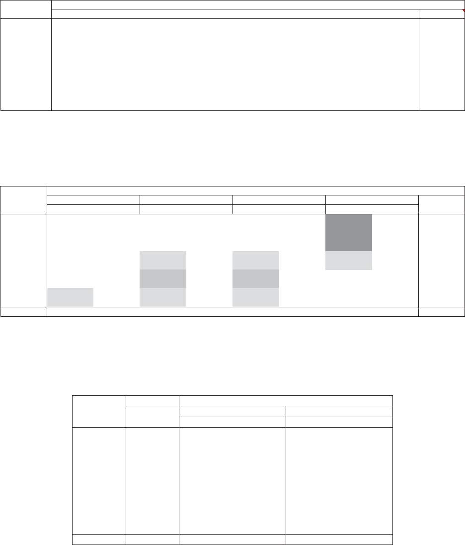
Casualty Actuarial Society 99
Using the ODP Bootstrap Model: A Practitioner’s Guide
Accident Model Weights by Accident Year
Year Paid CL Incd CL Paid BF Incd BF Paid CC Incd CC Paid GLM Incd GLM TOTAL
2006 100.0% 100.0%
2007 100.0% 100.0%
2008 100.0% 100.0%
2009 100.0% 100.0%
2010 33.3% 33.3% 33.3% 100.0%
2011 33.3% 33.3% 33.3% 100.0%
2012 50.0% 50.0% 100.0%
2013 50.0% 50.0% 100.0%
2014 33.3% 33.3% 33.3% 100.0%
2015 33.3% 33.3% 33.3% 100.0%
Figure C.17. Model Weights By Accident Year
Five Top 50 Companies
Schedule P, Part C – Commercial Auto Liability (in 000,000's)
Summary of Results by Model
Mean Estimated Unpaid
Accident Chain Ladder Bornhuetter-Ferguson Cape Cod GLM Bootstrap Best Est.
Year Paid Incurred Paid Incurred Paid Incurred Paid Incurred (Weighted)
2006 8115768810 8
2007 11 15 811913 14 17 13
2008 21 31 17 24 18 25 23 31 23
2009 35 53 35 49 36 52 38 54 38
2010 61 92 65 99 67 101 64 92 66
2011 110 168 123 176 124 183 123 174 124
2012 216 328 259 362 258 403 244 363 258
2013 410 623 481 642 481 696 457 682 480
2014 773 1,223 812 1,118 827 1,287 747 1,097 803
2015 1,103 1,513 1,132 1,554 1,178 1,647 1,063 1,567 1,134
Totals 2,746 4,056 2,936 4,040 3,004 4,415 2,781 4,087 2,947
Figure C.18. Estimated Mean Unpaid By Model
Five Top 50 Companies
Schedule P, Part C – Commercial Auto Liability (in 000,000's)
Summary of Results by Model
Ranges
Accident Best Est. Weighted Modeled
Year (Weighted) Minimum Maximum Mininum Maximum
2006 88858
2007 13 14 14
81
4
2008 23 23 23 17 23
2009 38 38 38 35 38
2010 66 64 67 61 67
2011 124 123 124 110 124
2012 258 258 259 216 259
2013 480 481 481 410 481
2014 803 773 827 747 827
2015 1,134 1,103 1,178 1,063 1,178
Totals 2,947 2,884 3,018 2,746 3,004
Figure C.19. Estimated Ranges

100 Casualty Actuarial Society
Using the ODP Bootstrap Model: A Practitioner’s Guide
Five Top 50 Companies
Schedule P, Part C – Commercial Auto Liability (in 000,000's)
Reconciliation of Total Results
Best Estimate (Weighted)
Accident Paid Incurred CaseEstimate of Estimate of
Year To Date To Date Reserves IBNR Ultimate Unpaid
2006 1,563 1,577 14 (6) 1,571 8
2007 1,469 1,505 36 (23) 1,482 13
2008 1,387 1,436 49 (26) 1,410 23
2009 1,350 1,417 67 (29) 1,388 38
2010 1,342 1,445 102 (37) 1,408 66
2011 1,198 1,345 147 (24) 1,321 124
2012 1,061 1,339 278 (20) 1,318 258
2013 853 1,327 474 6 1,333 480
2014 645 1,442 797 6 1,448 803
2015 294 1,422 1,128 6 1,428 1,134
Totals 11,162 14,255 3,093 (146) 14,109 2,947
Figure C.20. Reconciliation of Total Results (Weighted)
Five Top 50 Companies
Schedule P, Part C – Commercial Auto Liability (in 000,000's)
Accident Year Unpaid
Best Estimate (Weighted)
Accident Mean Standard Coefficient 50.0% 75.0% 95.0% 99.0%
Year Unpaid Error of Variation Minimum Maximum Percentile Percentile Percentile Percentile
2006 8565.8% (8) 35 7111
82
4
2007 13 7 51.3% (7) 52 13 17 26 33
2008 23 9 39.4% (5) 72 22 28 39 48
2009 38 11 28.9% 79237455
86
8
2010 66 12 17.8% 30 130 65 73 86 96
2011 124 22 17.6% 59 247 122 137 161 182
2012 258 40 15.4% 140 485 255 284 326 359
2013 480 47 9.8% 311 737 478 509 559 604
2014 803 65 8.1% 580 1,151 802 845 912 967
2015 1,134 83 7.3% 800 1,569 1,138 1,189 1,266 1,327
Totals 2,947 132 4.5% 2,471 3,532 2,947 3,036 3,162 3,257
Normal Dist. 2,947 132 4.5% 2,947 3,036 3,164 3,254
logNormal Dist. 2,947 132 4.5% 2,944 3,035 3,170 3,268
Gamma Dist. 2,947 132 4.5% 2,945 3,035 3,168 3,263
Figure C.21. Estimated Unpaid Model Results (Weighted)

Casualty Actuarial Society 101
Using the ODP Bootstrap Model: A Practitioner’s Guide
Five Top 50 Companies
Schedule P, Part C – Commercial Auto Liability (in 000,000's)
Calendar Year Unpaid
Best Estimate (Weighted)
Calendar Mean Standard Coefficient 50.0% 75.0% 95.0% 99.0%
Year Unpaid Error of Variation Minimum MaximumPercentile Percentile Percentile Percentile
2016 1,156 58 5.0% 937 1,3781,155 1,1941,254 1,299
2017 796 53 6.7% 611 993 795 832 886 927
2018 475 42 8.9% 332 668 474 503 547 580
2019 248 38 15.3% 129 410 246 273 315 342
2020 125 23 18.6% 60 260 123 139 165 187
2021 64 11 16.6% 25 110 63 71 82 91
2022 37 6 17.2% 15 71 37 41 48 53
2023 22 5 23.7% 55221253
03
5
2024 11 4 35.5% (1)3110131
72
1
2025 7343.3% -28791
31
6
2026 4253.2% -1
73579
2027 2169.8% -1
12246
2028 1195.7% -
91134
Totals 2,947 132 4.5% 2,471 3,5322,947 3,0363,162 3,257
Figure C.22. Estimated Cash Flow (Weighted)
Five Top 50 Companies
Schedule P, Part C – Commercial Auto Liability (in 000,000's)
Accident Year Ultimate Loss Ratios
Best Estimate (Weighted)
Accident Mean Standard Coefficient 50.0% 75.0% 95.0% 99.0%
Year Loss Ratio Error of Variation Minimum Maximum Percentile Percentile Percentile Percentile
2006 88.5% 2.7% 3.0% 79.6% 98.3% 88.5% 90.3% 92.9% 94.7%
2007 82.9% 2.5% 3.0% 73.9% 92.3% 82.9% 84.6% 87.0% 88.6%
2008 74.9% 2.3% 3.1% 65.8% 83.0% 74.9% 76.5% 78.7% 80.3%
2009 60.3% 1.9% 3.2% 52.4% 67.3% 60.4% 61.7% 63.5% 64.7%
2010 55.0% 2.1% 3.9% 47.5% 62.5% 55.0% 56.5% 58.4% 59.7%
2011 54.3% 1.9% 3.5% 46.8% 62.7% 54.4% 55.7% 57.5% 58.7%
2012 51.8% 2.0% 3.9% 44.0% 61.8% 51.8% 53.1% 55.2% 56.7%
2013 54.1% 2.3% 4.2% 46.9% 64.8% 54.1% 55.6% 57.9% 59.8%
2014 58.3% 2.8% 4.9% 48.6% 72.0% 58.3% 60.1% 63.0% 65.1%
2015 59.9% 3.6% 6.1% 45.7% 77.7% 60.1% 62.4% 65.7% 68.3%
Totals 62.4% 0.8% 1.3% 59.1% 65.8% 62.4% 63.0% 63.7% 64.3%
Figure C.23. Estimated Loss Ratio (Weighted)
Five Top 50 Companies
Schedule P, Part C – Commercial Auto Liability (in 000,000's)
Calendar Year Unpaid Claim Runoff
Best Estimate (Weighted)
Calendar Mean Standard Coefficient 50.0% 75.0% 95.0% 99.0%
Year Unpaid Error of Variation Minimum Maximum Percentile Percentile Percentile Percentile
2015 2,947 132 4.5% 2,471 3,532 2,947 3,036 3,162 3,257
2016 1,791 101 5.6% 1,449 2,233 1,790 1,859 1,959 2,027
2017 995 73 7.3% 739 1,286 993 1,043 1,117 1,170
2018 520 52 10.0% 345 712 518 554 608 649
2019 271 31 11.5% 161 415 270 291 325 352
2020 147 18 12.6% 65 246 146 159 178 193
2021 83 13 16.0% 31 156 82 91 106 116
2022 46 10 22.2% 11 97 45 53 63 71
2023 24 7 30.7% 16524293
74
4
2024 14 5 37.9% (0) 42 13 17 23 27
2025 6345.2% (0) 24 6811 14
2026 3260.2% (0) 13
2468
2027 1195.7% (0)
91134
2028 0019936.0% (0) 00000
Figure C.24. Estimated Unpaid Claim Runoff (Weighted)
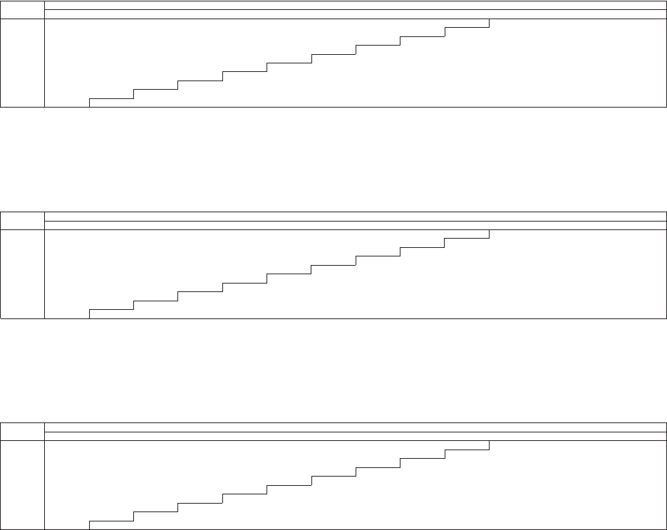
102 Casualty Actuarial Society
Using the ODP Bootstrap Model: A Practitioner’s Guide
Five Top 50 Companies
Schedule P, Part C – Commercial Auto Liability (in 000,000's)
Accident Year Incremental Values by Development Period
Best Estimate (Weighted)
Accident Mean Values
Year 12 24 36 48 60 72 84 96 108 120 132 144 156 168 +
2006 326 384 355 237 124 55 27 16 10
64211
2007 328 388 326 218 114 61 27 16
963211
2008 331 356 299 200 125 60 27 16
963211
2009 303 327 274 219 124 60 27 16
963211
2010 290 328 306 218 121 58 27 16 11
44211
2011 269 323 291 207 115 60 27 15 10
44211
2012 269 312 281 198 130 62 28 16 11
34211
2013 266 308 278 229 126 60 27 16 11
34211
2014 299 346 325 228 126 60 27 15 11
34211
2015 294 351 317 223 123 59 26 15 11 34211
Figure C.25. Mean of Incremental Values (Weighted)
Five Top 50 Companies
Schedule P, Part C – Commercial Auto Liability (in 000,000's)
Accident Year Incremental Values by Development Period
Best Estimate (Weighted)
Accident Standard Error Values
Year 12 24 36 48 60 72 84 96 108 120 132 144 156 168 +
2006 21 23 22 18 13
965433221
2007 21 23 21 17 13
965433221
2008 21 22 20 17 13
965433221
2009 21 21 19 17 13
965433221
2010 18 26 23 14 22 15
84432211
2011 18 17 22 15 22 18
84432211
2012 13 14 22 11 30 21
84322111
2013 13 14 22 18 31 21
84322111
2014 13 14 33 18 30 21
84322111
2015 13 26 32 19 30 21
84322111
Figure C.26. Standard Deviation of Incremental Values (Weighted)
Five Top 50 Companies
Schedule P, Part C – Commercial Auto Liability (in 000,000's)
Accident Year Incremental Values by Development Period
Best Estimate (Weighted)
Accident Coefficients of Variation
Year 12 24 36 48 60 72 84 96 108 120 132 144 156 168 +
2006 6.5% 6.0% 6.2% 7.6% 10.4% 15.9% 22.6% 29.2% 37.6% 49.0% 74.6% 95.5% 122.0%
156.9%
2007 6.4% 5.9% 6.5% 8.0% 11.0% 15.0% 22.4% 28.9% 38.1% 56.2% 73.4% 94.7% 123.1%
157.6%
2008 6.5% 6.2% 6.8% 8.3% 10.4% 15.0% 22.6% 29.3% 41.7% 56.2% 73.4% 95.5% 122.4%
160.6%
2009 6.8% 6.4% 7.1% 7.9% 10.6% 15.2% 22.7% 31.5% 42.2% 56.9% 74.2% 96.8% 121.7%
162.3%
2010 6.1% 7.9% 7.3% 6.3% 18.2% 25.8% 28.6% 26.8% 35.0% 65.1% 63.8% 81.4% 111.5%
113.7%
2011 6.6% 5.4% 7.6% 7.2% 18.7% 30.1% 29.0% 27.1% 34.8% 66.8% 64.0% 82.4% 113.2%
115.9%
2012 4.8% 4.5% 7.8% 5.6% 23.4% 34.1% 30.0% 24.4% 30.1% 60.7% 57.6% 71.7% 93.4%
94.2%
2013 4.8% 4.4% 7.9% 7.9% 24.2% 34.5% 30.4% 24.4% 30.2% 61.4% 58.2% 72.2% 94.5%
94.4%
2014 4.5% 4.2% 10.0% 8.1% 23.6% 34.6% 30.2% 24.7% 30.3% 62.0% 59.4% 73.2% 94.7%
95.6%
2015 4.6% 7.4% 10.0% 8.3% 24.3% 35.0% 31.0% 24.6% 30.6% 61.4% 59.9% 73.5% 97.0%
95.7%
Figure C.27. Coefficient of Variation of Incremental Values (Weighted)
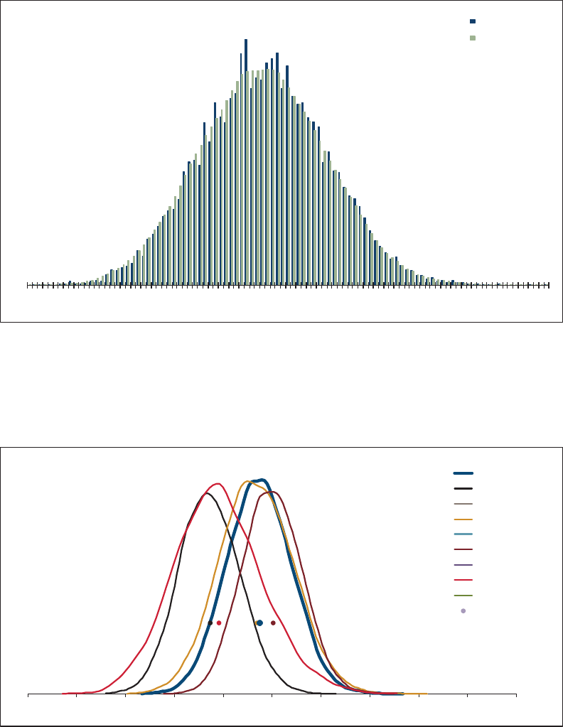
Casualty Actuarial Society 103
Using the ODP Bootstrap Model: A Practitioner’s Guide
Five Top 50 Companies
Schedule P, Part C – Commercial Auto Liability (in 000,000's)
Total Unpaid Distribution
Best Estimate (Weighted)
2.5K 2.6K 2.7K 2.8K 2.9K 3.0K 3.1K 3.2K 3.3K 3.4K 3.5K
Probability
Total Unpaid
Histogram
Kernel Density
Figure C.28. Total Unpaid Claims Distribution (Weighted)
Five Top 50 Companies
Schedule P, Part C – Commercial Auto Liability (in 000,000's)
Summary of Model Distributions
(Using Kernel Densities)
2.0K 2.2K 2.4K 2.6K 2.8K 3.0K 3.2K 3.4K 3.6K 3.8K 4.0K
Probability
Total Unpaid
Best Estimate
Paid CL
Incurred CL
Paid BF
Incurred BF
Paid CC
Incurred CC
Paid GLM
Incurred GLM
Mean Estimates
Figure C.29. Summary of Model Distributions

104 Casualty Actuarial Society
Appendix D—Aggregate Results
In this appendix the results for the correlated aggregate of the three Schedule P lines of
business (Parts A, B, and C) are shown, using the correlation calculated from the paid
data after adjustment for heteroscedasticity.
Five Top 50 Companies
Aggregate Three Lines of Business
Accident Year Unpaid
Accident Mean Standard Coefficient 50.0% 75.0% 95.0% 99.0%
Year Unpaid Error of Variation Minimum Maximum Percentile Percentile Percentile Percentile
2006 67 25 37.9% 0 186 66 83 110 130
2007 107 30 28.1% 25 295 105 126 158 185
2008 199 49 24.8% 67 622 194 226 285 342
2009 298 56 18.8% 123 800 293 331 395 457
2010 480 69 14.3% 248 959 475 522 599 668
2011 862 106 12.3% 503 1,561 860 923 1,041 1,135
2012 1,666 187 11.2% 383 2,555 1,662 1,771 1,985 2,148
2013 3,070 333 10.8% 1,808 6,522 3,066 3,249 3,649 3,928
2014 5,632 703 12.5% 2,435 8,555 5,632 6,075 6,801 7,326
2015 13,270 1,788 13.5% 5,217 22,660 13,262 14,348 16,180 18,011
Totals 25,650 2,080 8.1% 16,952 36,085 25,616 26,949 29,088 30,991
Normal Dist. 25,650 2,080 8.1% 25,650 27,053 29,072 30,490
logNormal Dist. 25,650 2,088 8.1% 25,566 27,006 29,222 30,885
Gamma Dist. 25,650 2,080 8.1% 25,594 27,021 29,165 30,736
Figure D.1. Estimated Unpaid Model Results
Five Top 50 Companies
Aggregate Three Lines of Business
Calendar Year Unpaid
Calendar Mean Standard Coefficient 50.0% 75.0% 95.0% 99.0%
Year Unpaid Error of Variation Minimum Maximum Percentile Percentile Percentile Percentile
2016 12,906 1,209 9.4% 8,242 19,475 12,869 13,611 14,897 16,182
2017 5,733 453 7.9% 3,991 7,589 5,727 6,024 6,488 6,836
2018 3,144 257 8.2% 2,132 4,373 3,137 3,310 3,573 3,781
2019 1,663 144 8.6% 1,163 2,415 1,657 1,757 1,906 2,018
2020 903 86 9.5% 617 1,331 900 958 1,050 1,122
2021 512 59 11.5% 319 1,064 508 546 613 678
2022 324 55 16.9% 140 699 317 353 423 484
2023 217 64 29.4% 86 931 205 245 328 431
2024 120 28 23.7% 21 308 118 137 170 197
2025 74 22 30.1% 7 165 73 89 113 131
2026 36 13 37.2% 29435455
97
0
2027 18 9 51.9% 05817243
34
1
2028 1195.7% -
91134
Totals 25,650 2,080 8.1% 16,952 36,085 25,616 26,949 29,088 30,991
Figure D.2. Estimated Cash Flow
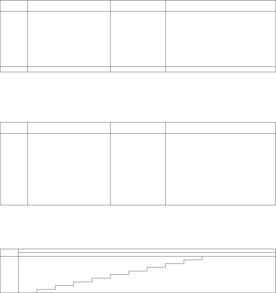
Casualty Actuarial Society 105
Using the ODP Bootstrap Model: A Practitioner’s Guide
Five Top 50 Companies
Aggregate Three Lines of Business
Accident Year Ultimate Loss Ratios
AccidentMean Standard Coefficient 50.0% 75.0% 95.0% 99.0%
Year Loss Ratio Error of Variation Minimum MaximumPercentile Percentile Percentile Percentile
2006 74.0% 10.7% 14.5% 33.5% 132.5% 73.7% 77.5% 93.7% 109.6%
2007 81.3% 11.5% 14.2% 38.3% 147.1% 81.0% 85.0% 102.0% 121.0%
2008 85.4% 11.8% 13.8% 39.5% 153.1% 85.0% 89.2% 107.7% 123.9%
2009 76.0% 10.2% 13.4% 36.8% 131.0% 75.6% 79.4% 94.7% 111.2%
2010 66.9% 9.3% 13.9% 31.0% 119.9% 66.3% 70.1% 84.1% 97.9%
2011 64.5% 8.9% 13.8% 30.1% 117.2% 64.2% 67.5% 81.1% 91.4%
2012 71.0% 10.1% 14.3% 31.6% 129.3% 70.5% 74.0% 90.5% 104.6%
2013 61.4% 8.5% 13.9% 29.3% 125.5% 61.1% 64.2% 77.3% 88.8%
2014 65.4% 9.7% 14.8% 31.3% 115.9% 65.2% 70.3% 82.2% 94.9%
2015 78.2% 11.5% 14.7% 39.0% 143.2% 77.8% 83.8% 97.6% 113.8%
Totals 71.6% 3.3% 4.6% 59.5% 88.1% 71.5% 73.7% 77.3% 80.3%
Figure D.3. Estimated Loss Ratio
Five Top 50 Companies
Aggregate Three Lines of Business
Calendar Year Unpaid Claim Runoff
Calendar Mean Standard Coefficient 50.0%75.0% 95.0%99.0%
Year UnpaidError of Variation Minimum Maximum Percentile Percentile Percentile Percentile
2015 25,650 2,080 8.1% 16,952 36,085 25,616 26,949 29,088 30,991
2016 12,744 944 7.4% 8,710 17,043 12,733 13,373 14,296 15,047
2017 7,012 536 7.6% 4,664 9,5517,000 7,3687,905 8,324
2018 3,868 319 8.2% 2,512 5,3883,861 4,0754,406 4,671
2019 2,205 213 9.7% 1,348 3,2592,196 2,3402,567 2,762
2020 1,302 158 12.1% 730 2,2661,292 1,4001,574 1,733
2021 790 126 15.9% 401 1,697781 8641,003 1,145
2022 466 99 21.2% 166 1,272458 524636 746
2023 249 62 24.9% 45 533245 289359 403
2024 129 42 32.4% 13 294126 156202 236
2025 55 21 37.9% 3141 53 68 90 107
2026 19 9 49.6% 06018253
44
2
2027 1195.7% (0) 91134
Figure D.4. Estimated Unpaid Claim Runoff
Five Top 50 Companies
Aggregate Three Lines of Business
Accident Year Incremental Values by Development Period
Accident Mean Values
Year 12 24 36 48 60 72 84 96 108 120 132 144 156 168 +
2006 9,334 4,878 2,029 1,175 621 300 151 79 67 33 33 17 16 1
2007 10,595 5,394 2,159 1,239 655 327 163 85 75 35 35 18 17 1
2008 12,060 5,959 2,317 1,321 716 352 175 91 84 38 38 19 18 1
2009 11,848 6,007 2,371 1,389 745 365 182 95 83 40 40 20 20 1
2010 11,834 5,923 2,345 1,351 721 354 182 95 85 38 40 20 19 1
2011 12,195 5,972 2,312 1,326 707 372 185 96 90 39 40 20 19 1
2012 14,186 6,541 2,409 1,362 775 380 191 99 103 39 40 20 19 1
2013 11,901 5,868 2,282 1,436 763 374 187 97 93 38 40 20 19 1
2014 12,949 6,354 2,538 1,451 771 378 189 98 98 38 36 19 17 1
2015 16,458 7,356 2,685 1,515 794 395 202 108 99 44 36 19 17 1
Figure D.5. Mean of Incremental Values
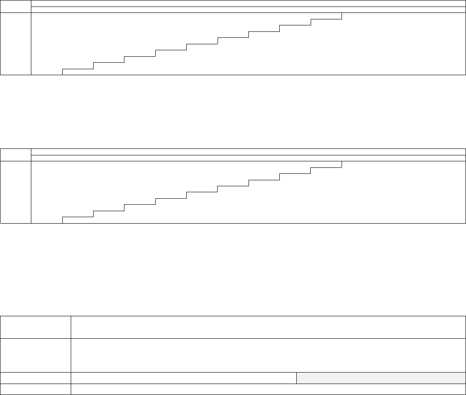
106 Casualty Actuarial Society
Using the ODP Bootstrap Model: A Practitioner’s Guide
Five Top 50 Companies
Aggregate Three Lines of Business
Accident Year Incremental Values by Development Period
Accident Standard Deviation Values
Year 12 24 36 48 60 72 84 96 108120 132144 15
61
68 +
2006 1,735 668 233 134 74 37 18 13 23 61
3766
2007 1,909 712 244 140 77 39 18 14 26 10 14 7710
2008 2,085 768 264 147 81 41 20 14 35 11 15 8711
2009 2,010 754 260 149 82 41 19 17 34 10 15 8810
2010 2,059 775 264 148 84 43 22 17 35 11 15 8811
2011 2,085 777 261 150 84 49 22 17 37 11 16 8811
2012 2,492 875 277 155 98 50 23 17 44 12 15 8812
2013 2,078 767 261 169 97 51 23 17 39 11 15 8811
2014 2,300 907 341 192 109 55 26 19 42 13 17 9913
2015 2,728 1,087 365 210 116 59 30 23 58 17 17 9917
Figure D.6. Standard Deviation of Incremental Values
Five Top 50 Companies
Aggregate Three Lines of Business
Accident Year Incremental Values by Development Period
Accident Coefficients of Variation
Year 12 24 36 48 60 72 84 96 108 120 132 144 156 168 +
2006 18.6% 13.7% 11.5% 11.4% 11.9% 12.5% 11.7% 16.8% 35.0% 17.0% 38.4% 38.5% 40.0%
702.6%
2007 18.0% 13.2% 11.3% 11.3% 11.8% 12.0% 11.4% 16.3% 35.1% 27.8% 38.5% 38.6% 40.0%
1216.6%
2008 17.3% 12.9% 11.4% 11.1% 11.3% 11.7% 11.2% 15.7% 42.1% 28.0% 39.1% 39.2% 40.5%
1356.5%
2009 17.0% 12.6% 11.0% 10.7% 11.0% 11.3% 10.7% 17.7% 41.4% 26.2% 38.8% 39.0% 40.2%
1287.1%
2010 17.4% 13.1% 11.3% 11.0% 11.6% 12.2% 11.9% 17.7% 40.5% 27.6% 39.0% 39.4% 40.8%
1164.5%
2011 17.1% 13.0% 11.3% 11.3% 11.9% 13.3% 11.9% 17.5% 41.5% 28.2% 39.2% 39.5% 40.9%
1219.1%
2012 17.6% 13.4% 11.5% 11.4% 12.6% 13.2% 12.0% 16.9% 42.8% 31.6% 38.6% 39.0% 40.6%
1268.9%
2013 17.5% 13.1% 11.4% 11.8% 12.6% 13.6% 12.1% 17.3% 41.9% 29.1% 38.5% 38.9% 40.4%
1214.5%
2014 17.8% 14.3% 13.5% 13.3% 14.2% 14.5% 13.8% 19.0% 43.0% 34.8% 47.6% 46.7% 54.6%
1429.6%
2015 16.6% 14.8% 13.6% 13.8% 14.6% 15.0% 14.9% 21.5% 58.1% 38.8% 47.3% 46.7% 54.4% 1901.0%
Figure D.7. Coefficient of Variation of Incremental Values
Five Top 50 Companies
Aggregate Three Lines of Business
Indicated Unpaid Claim Risk Portion of Required Capital
Earned Mean 99.0% Value at Risk Allocated Unpaid Premium
LOB / Segment Premium Unpaid Unpaid CapitalCapitalRatio Ratio
Schedule P, Part A 15,148 5,308 8,675 3,367 2,642 49.8% 17.4%
Schedule P, Part B 20,467 17,395 20,525 3,130 2,456 14.1% 12.0%
Schedule P, Part C 2,383 2,947 3,257 310 243 8.3% 10.2%
Total 37,997 25,650 32,457 6,807
Aggregate 37,997 25,650 30,991 5,341 5,341 20.8% 14.1%
Figure D.8. Calculation of Risk Based Capital
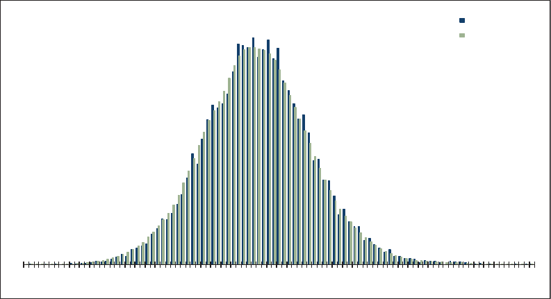
Casualty Actuarial Society 107
Using the ODP Bootstrap Model: A Practitioner’s Guide
Five Top 50 Companies
Aggregate Three Lines of Business
Total Unpaid Distribution
16.9K
18.8K 20.7K 22.7K 24.6K 26.5K 28.4K30.4K 32.3K 34.2K 36.1K
Probability
Total Unpaid
Histogram
Kernel Density
Figure D.9. Total Unpaid Claims Distribution

108 Casualty Actuarial Society
Appendix E—GLM Bootstrap Results
In this appendix the results for the GLM Bootstrap model, as illustrated in Figures 5.9
through 5.12 using the Taylor and Ashe (1983) data, are shown.
Taylor and Ashe Data
Accident Year Unpaid
Paid GLM Bootstrap Model
Accident Mean Standard Coefficient 50.0% 75.0% 95.0% 99.0%
Year Unpaid Error of Variation Minimum MaximumPercentilePercentilePercentilePercentile
2006 --
------
2007 201,062 86,944 43.2% 13,857 542,484 186,940 254,238 361,288 438,224
2008 438,222 193,377 44.1% 48,640 1,570,379 405,070 547,131 798,395 996,074
2009 701,223 229,176 32.7% 192,462 1,747,698 679,682 831,657 1,122,868 1,320,964
2010 1,024,913 264,752 25.8% 405,036 2,286,536 1,009,377 1,186,714 1,467,758 1,825,411
2011 1,452,650 315,901 21.7% 619,534 2,544,116 1,424,030 1,660,714 1,996,927 2,261,272
2012 2,181,115 481,962 22.1% 916,307 4,248,064 2,136,166 2,480,213 3,027,607 3,396,995
2013 3,468,030 603,268 17.4% 1,751,033 5,598,537 3,424,738 3,862,292 4,553,992 4,965,982
2014 4,568,990 695,194 15.2% 2,331,572 6,824,685 4,526,036 5,039,460 5,731,706 6,408,694
2015 5,672,877 744,661 13.1% 3,681,244 8,333,062 5,657,952 6,171,074 6,954,411 7,414,615
Totals 19,709,081 2,176,864 11.0% 13,360,401 27,429,908 19,594,207 21,069,822 23,354,466 24,752,422
Normal Dist. 19,709,081 2,176,864 11.0% 19,709,081 21,177,353 23,289,703 24,773,224
logNormal Dist. 19,709,844 2,194,514 11.1% 19,588,799 21,111,651 23,512,537 25,360,134
Gamma Dist. 19,709,081 2,176,864 11.0% 19,628,994 21,130,455 23,421,097 25,123,713
Figure E.1. Estimated Unpaid Model Results
Taylor and Ashe Data
Calendar Year Unpaid
Paid GLM Bootstrap Model
CalendarMean Standard Coefficient 50.0% 75.0% 95.0% 99.0%
Year Unpaid Errorof Variation Minimum Maximum Percentile Percentile Percentile Percentile
2016 5,367,217 639,639 11.9% 3,363,8637,428,225 5,343,203 5,770,597 6,447,544 6,986,539
2017 4,312,360 599,300 13.9% 2,363,7046,455,658 4,279,059 4,673,264 5,338,534 5,922,511
2018 3,310,498 539,509 16.3% 1,993,1075,419,760 3,288,209 3,657,889 4,209,239 4,690,515
2019 2,245,627 417,764 18.6% 1,078,0004,088,770 2,221,086 2,510,176 2,948,019 3,475,039
2020 1,676,436 369,916 22.1% 619,943 3,157,564 1,644,779 1,921,249 2,318,054 2,614,635
2021 1,224,109 326,624 26.7% 444,913 2,352,525 1,202,484 1,436,029 1,782,066 2,085,204
2022 838,442 264,751 31.6% 226,969 2,477,444 803,316 991,076 1,302,125 1,532,640
2023 507,334 211,762 41.7% 104,873 1,268,302 480,233 635,243 889,537 1,135,405
2024 227,058 93,270 41.1% 32,667 711,619 213,471 277,710 403,483 498,676
2025 -- -
-----
Totals 19,709,081 2,176,86411.0% 13,360,401 27,429,908 19,594,207 21,069,822 23,354,466 24,752,422
Figure E.2. Estimated Cash Flow
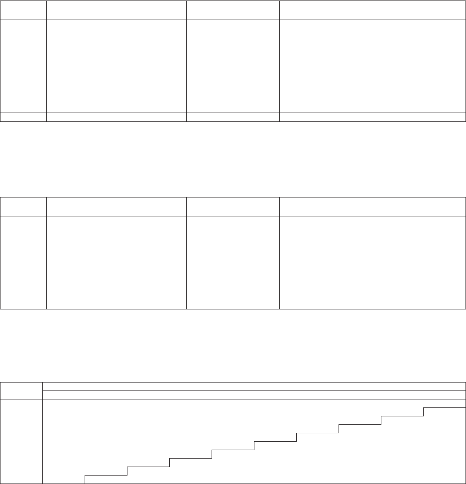
Casualty Actuarial Society 109
Using the ODP Bootstrap Model: A Practitioner’s Guide
Taylor and Ashe Data
Accident Year Ultimate Loss Ratios
Paid GLM Bootstrap Model
AccidentMean Standard Coefficient 50.0% 75.0%95.0% 99.0%
Year Loss RatioError of Variation Minimum Maximum Percentile Percentile Percentile Percentile
2006 54.8% 6.4% 11.7% 38.1% 74.0% 54.7% 59.0% 65.7% 70.4%
2007 65.0% 6.4% 9.8% 48.1% 84.1% 65.0% 68.9% 75.7% 80.7%
2008 63.1% 6.4% 10.1% 42.6% 82.0% 63.1% 67.3% 73.4% 78.6%
2009 56.0% 6.2% 11.0% 38.0% 76.4% 55.9% 60.0% 66.2% 71.6%
2010 53.1% 5.9% 11.0% 34.7% 74.7% 52.8% 57.1% 63.1% 66.6%
2011 50.5% 5.6% 11.1% 33.9% 70.0% 50.2% 54.2% 60.0% 63.9%
2012 53.8% 7.6% 14.2% 31.3% 81.3% 53.1% 59.1% 66.8% 72.8%
2013 55.3% 6.9% 12.5% 34.6% 78.4% 55.1% 59.5% 66.9% 73.4%
2014 52.9% 6.8% 12.8% 31.7% 74.5% 52.4% 57.2% 64.5% 70.1%
2015 50.7% 6.5% 12.8% 33.0% 72.4% 50.6% 55.1% 61.6% 65.8%
Totals 55.1% 2.9% 5.2% 46.9% 63.6% 55.1% 57.1% 60.0% 61.7%
Figure E.3. Estimated Loss Ratio
Taylor and Ashe Data
Calendar Year Unpaid Claim Runoff
Paid GLM Bootstrap Model
Calendar Mean Standard Coefficient 50.0% 75.0% 95.0% 99.0%
Year UnpaidError of VariationMinimum Maximum Percentile Percentile Percentile Percentile
2015 19,709,081 2,176,864 11.0% 13,360,401 27,429,908 19,594,207 21,069,822 23,354,466 24,752,422
2016 14,341,864 1,839,659 12.8% 8,990,374 21,139,070 14,231,008 15,525,987 17,412,102 19,106,264
2017 10,029,504 1,499,062 14.9% 5,923,686 15,623,104 9,926,619 10,979,472 12,605,655 13,627,923
2018 6,719,006 1,188,158 17.7% 3,317,118 11,201,515 6,612,903 7,438,758 8,841,160 9,734,081
2019 4,473,380 922,335 20.6% 1,884,408 7,436,971 4,366,371 5,040,244 6,143,079 6,968,601
2020 2,796,943 678,192 24.2% 1,137,743 5,050,304 2,740,868 3,192,138 4,018,580 4,623,373
2021 1,572,834 443,756 28.2% 595,162 3,523,942 1,524,022 1,852,397 2,369,545 2,820,528
2022 734,392 257,467 35.1% 204,545 1,654,724 708,577 888,204 1,167,670 1,463,534
2023 227,058 93,270 41.1% 32,667 711,619 213,471 277,710 403,483 498,676
2024 004017.8% (0)0-000
Figure E.4. Estimated Unpaid Claim Runoff
Taylor and Ashe Data
Accident Year Incremental Values by Development Period
Paid GLM Bootstrap Model
Accident Mean Values
Year 12 24 36 48 60 72 84 96 108 120+
2006 260,293 698,693 688,850 704,606 388,809 311,880 258,794 214,532 169,749 142,707
2007 353,111 978,505 972,391 972,627 539,441 447,302 359,572 300,611 234,076 201,062
2008 355,598 975,396 989,087 971,633 541,986 440,002 357,470 297,335 237,981 200,241
2009 343,575 914,108 911,442 913,681 502,676 421,801 335,888 282,854 231,129 187,240
2010 341,295 923,102 914,709 919,809 500,195 420,057 337,719 275,372 224,883 186,939
2011 336,529 924,119 917,372 913,328 503,784 409,092 338,662 284,360 234,436 186,099
2012 381,818 1,028,561 1,036,624 1,025,187 578,558 451,767 374,253 312,453 251,461 212,623
2013 402,258 1,107,072 1,108,427 1,111,762 614,292 501,712 410,170 332,713 265,392 231,989
2014 408,511 1,104,124 1,109,649 1,096,598 616,324 491,960 408,977 338,285 274,715 232,482
2015 406,207 1,098,540 1,104,298 1,121,727 609,668 497,186 407,810 331,738 274,852 227,058
Figure E.5. Mean of Incremental Values
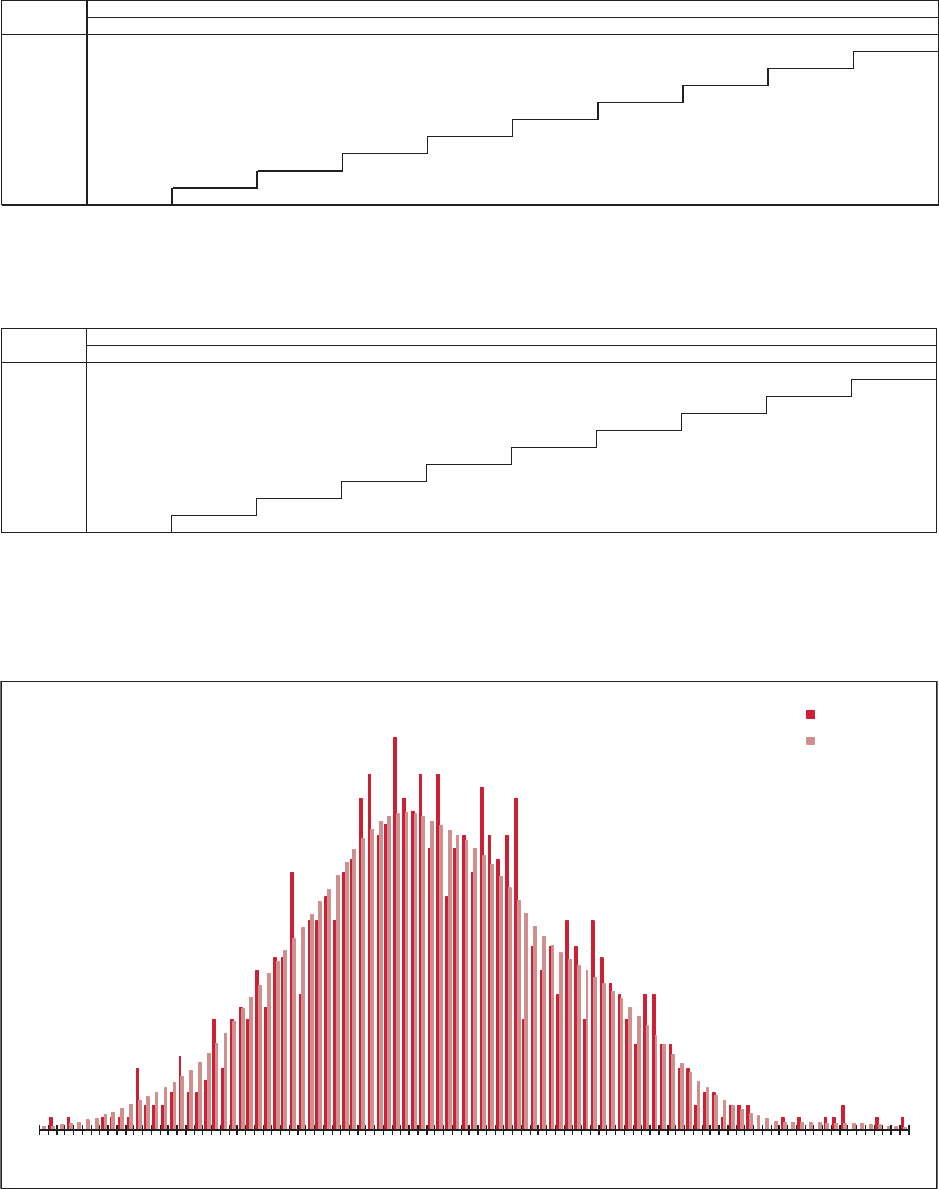
110 Casualty Actuarial Society
Using the ODP Bootstrap Model: A Practitioner’s Guide
Taylor and Ashe Data
Accident Year Incremental Values by Development Period
Paid GLM Bootstrap Model
Accident Standard Error Values
Year 12 24 36 48 60 72 84 96 108 120+
2006 108,496 120,663 181,091 248,062 129,788 119,862 108,476 67,654 126,590 56,408
2007 131,381 142,390 209,358 306,437 159,961 138,486 133,743 80,122 152,143 86,944
2008 127,448 146,072 215,044 306,874 152,841 142,207 122,350 78,132 159,664 86,683
2009 125,340 137,368 201,409 295,530 154,057 138,440 121,788 90,057 156,660 80,901
2010 127,558 139,764 193,891 297,664 152,539 136,999 129,441 88,860 139,515 78,776
2011 125,839 139,522 196,494 285,649 156,869 139,339 128,102 92,988 160,838 81,152
2012 137,400 150,449 208,476 321,223 187,435 156,077 150,736 103,377 165,336 93,178
2013 137,189 150,565 221,025 338,863 195,056 173,394 151,060 103,542 169,356 96,165
2014 132,459 159,062 254,892 329,254 195,407 162,115 149,531 106,739 171,923 94,787
2015 135,172 183,619 247,413 336,959 177,810 163,745 147,122 102,400 167,873 93,270
Figure E.6. Standard Deviation of Incremental Values
Taylor and Ashe Data
Accident Year Incremental Values by Development Period
Paid GLM Bootstrap Model
AccidentCoefficient of Variation Values
Year 12 24 36 48 60 72 84 96 10
81
20+
2006 41.7% 17.3% 26.3% 35.2% 33.4% 38.4% 41.9% 31.5% 74.6% 39.5%
2007 37.2% 14.6% 21.5% 31.5% 29.7% 31.0% 37.2% 26.7% 65.0% 43.2%
2008 35.8% 15.0% 21.7% 31.6% 28.2% 32.3% 34.2% 26.3% 67.1% 43.3%
2009 36.5% 15.0% 22.1% 32.3% 30.6% 32.8% 36.3% 31.8% 67.8% 43.2%
2010 37.4% 15.1% 21.2% 32.4% 30.5% 32.6% 38.3% 32.3% 62.0% 42.1%
2011 37.4% 15.1% 21.4% 31.3% 31.1% 34.1% 37.8% 32.7% 68.6% 43.6%
2012 36.0% 14.6% 20.1% 31.3% 32.4% 34.5% 40.3% 33.1% 65.8% 43.8%
2013 34.1% 13.6% 19.9% 30.5% 31.8% 34.6% 36.8% 31.1% 63.8% 41.5%
2014 32.4% 14.4% 23.0% 30.0% 31.7% 33.0% 36.6% 31.6% 62.6% 40.8%
2015 33.3% 16.7% 22.4% 30.0% 29.2% 32.9% 36.1% 30.9% 61.1% 41.1%
Figure E.7. Coefficient of Variation of Incremental Values
Taylor and Ashe Data
Total Unpaid Distribution
Paid GLM Bootstrap Model
13.3M 14.7M 16.1M 17.6M 19.0M 20.4M 21.8M 23.2M 24.6M 26.1M 27.5M
Probability
Total Unpaid
Histogram
Kernel Density
Figure E.8. Total Unpaid Claims Distribution
Casualty Actuarial Society 111
References
Anderson, Duncan, Sholom Feldblum, Claudine Modlin, Doris Schirmacher, Ernesto
Schirmacher, and Neeza andi. 2007. “A Practitioner’s Guide to Generalized
Linear Models,” CAS Exam Study Note, 3rd Edition: 1–116.
Ashe, Frank. 1986. “An Essay at Measuring the Variance of Estimates of Outstanding
Claim Payments.” ASTIN Bulletin 16:S: 99–113.
Barnett, Glen, and Ben Zehnwirth. 2000. “Best Estimates for Reserves.” Proceedings of
the Casualty Actuarial Society 87, 2: 245–321.
Berquist, James R., and Richard E. Sherman. 1977. “Loss Reserve Adequacy Testing: A
Comprehensive, Systematic Approach.” Proceedings of the Casualty Actuarial Society
64: 123–184.
Bornhuetter, Ronald, and Ronald Ferguson. 1972. “e Actuary and IBNR.” Proceed-
ings of the Casualty Actuarial Society 59: 181–195.
CAS Loss Simulation Model Working Party Summary Report. 2011. “Modeling Loss
Emergence and Settlement Processes.” Casualty Actuarial Society Forum (Winter) 1:
1–124.
CAS Working Party on Quantifying Variability in Reserve Estimates. 2005. “e
Analysis and Estimation of Loss & ALAE Variability: A Summary Report.” Casu-
alty Actuarial Society Forum (Fall): 29–146.
CAS Tail Factor Working Party. 2013. “e Estimation of Loss Development Tail Fac-
tors: A Summary Report.” Casualty Actuarial Society E-Forum (Fall): 1–111.
Christofides, S. 1990. “Regression Models Based on Log-Incremental Payments.”
Claims Reserving Manual, vol. 2. Institute of Actuaries, London.
Efron, Bradley. 1979. “Bootstrap Methods: Another Look at the Jackknife.” e Annals
of Statistics 7-1: 1–26.
England, Peter D., and Richard J. Verrall. 1999. “Analytic and Bootstrap Estimates of
Prediction Errors in Claims Reserving.” Insurance: Mathematics and Economics 25:
281–293.
England, Peter D., and Richard J. Verrall. 2002. “Stochastic Claims Reserving in Gen-
eral Insurance.” British Actuarial Journal 8-3: 443–544.
England, Peter D., and Richard J. Verrall. 2006. “Predictive Distributions of Out-
standing Liabilities in General Insurance.” e Annals of Actuarial Science 1, 2:
221–270.
11 2 Casualty Actuarial Society
Using the ODP Bootstrap Model: A Practitioner’s Guide
Foundations of Casualty Actuarial Science, 4th ed. 2001. Arlington, Va.: Casualty Actu-
arial Society.
Iman, R., and W. Conover. 1982. “A Distribution-Free Approach to Inducing Rank
Correlation Among Input Variables.” Communications in Statistics—Simulation and
Computation 11(3): 311–334.
IAA (International Actuarial Association). 2010. “Stochastic Modeling—eory
and Reality from an Actuarial Perspective.” Available from www.actuaries.org/
stochastic.
Kirschner, Gerald S., Colin Kerley, and Belinda Isaacs. 2008. “Two Approaches to
Calculating Correlated Reserve Indications Across Multiple Lines of Business.”
Variance 1: 15–38.
Kremer, E. 1982. “IBNR Claims and the Two Way Model of ANOVA” Scandinavian
Actuarial Journal: 47–55.
Liu, H., and R. Verrall. 2010. “Bootstrap Estimation of the Predictive Distributions of
Reserves Using Paid and Incurred Claims.” Variance 4: 125–135.
McCullagh, P., and J. Nelder. 1989. Generalized Linear Models, 2nd ed. Chapman
and Hall.
Mildenhall, Stephen J. 2006. “Correlation and Aggregate Loss Distributions with
an Emphasis on the Iman-Conover Method.” Casualty Actuarial Society E-Forum
(Winter): 103–204.
Milliman. 2014. “Using the Milliman Arius Reserving Model.” Version 2.1.
Pinheiro, Paulo J. R., João Manuel Andrade e Silva, and Maria de Lourdes Centeno.
2001. “Bootstrap Methodology in Claim Reserving.” ASTIN Colloquium: 1–13.
Pinheiro, Paulo J. R., João Manuel Andrade e Silva, and Maria de Lourdes Centeno.
2003. “Bootstrap Methodology in Claim Reserving.” Journal of Risk and Insur-
ance 70: 701–714.
Quarg, Gerhard, and omas Mack. 2008. “Munich Chain Ladder: A Reserving Method
that Reduces the Gap between IBNR Projections Based on Paid Losses and IBNR
Projections Based on Incurred Losses.” Variance 2: 266–299.
ROC/GIRO Working Party. 2007. “Best Estimates and Reserving Uncertainty.” Insti-
tute of Actuaries.
ROC/GIRO Working Party. 2008. “Reserving Uncertainty.” Institute of Actuaries.
Renshaw, A. E., 1989. “Chain Ladder and Interactive Modelling (Claims Reserving
and GLIM).” Journal of the Institute of Actuaries 116 (III): 559–587.
Renshaw, A. E., and R. J. Verrall. 1994. “A Stochastic Model Underlying the Chain
Ladder Technique.” Proceedings XXV ASTIN Colloquium, Cannes.
Struzzieri, Paul J., and Paul R. Hussian. 1998. “Using Best Practices to Determine a
Best Reserve Estimate.” Casualty Actuarial Society Forum (Fall): 353–413.
Taylor, Greg, and Frank Ashe. 1983. “Second Moments of Estimates of Outstanding
Claims.” Journal of Econometrics 23-1: 37–61.
Venter, Gary G. 1998. “Testing the Assumptions of Age-to-Age Factors.” Proceedings of
the Casualty Actuarial Society 85: 807–47.
Casualty Actuarial Society 11 3
Using the ODP Bootstrap Model: A Practitioner’s Guide
Verrall, Richard J. 1991. “On the Estimation of Reserves from Loglinear Models.”
Insurance: Mathematics and Economics 10: 75–80.
Verrall, Richard J. 2004. “A Bayesian Generalized Linear Model for the Bornhuetter-
Ferguson Method of Claims Reserving.” North American Actuarial Journal 8-3: 67–89.
Zehnwirth, Ben, 1989. “e Chain Ladder Technique—A Stochastic Model.” Claims
Reserving Manual vol. 2. Institute of Actuaries, London.
Zehnwirth, Ben. 1994. “Probabilistic Development Factor Models with Applications
to Loss Reserve Variability, Prediction Intervals and Risk Based Capital.” Casualty
Actuarial Society Forum (Spring), 2: 447–606.
114 Casualty Actuarial Society
Selected Bibliography
Björkwall, Susanna. 2009. “Bootstrapping for Claims Reserve Uncertainty in General
Insurance.” Mathematical Statistics, Stockholm University. Research Report 2009:3,
Licenciate thesis. http://www2.math.su.se/matstat/reports/seriea/2009/rep3/
report.pdf.
Björkwall, Susanna, Ola Hössjer, and Esbjörn Ohlsson. 2009. “Non-parametric and
Parametric Bootstrap Techniques for Age-to-Age Development Factor Methods in
Stochastic Claims Reserving.” Scandinavian Actuarial Journal 4: 306–331.
Freedman, D. A. 1981. “Bootstrapping Regression Models.” e Annals of Statistics
9-6: 1218–1228.
Hayne, Roger M. 2008. “A Stochastic Framework for Incremental Average Reserve
Models.” Casualty Actuarial Society E-Forum (Fall): 174–195.
Mack, omas. 1993. “Distribution Free Calculation of the Standard Error of Chain
Ladder Reserve Estimates.” ASTIN Bulletin 23-2: 213–225.
Mack, omas. 1999. “e Standard Error of Chain Ladder Reserve Estimates: Recur-
sive Calculation and Inclusion of a Tail Factor.” ASTIN Bulletin 29-2: 361–366.
Mack, omas, and Gary Venter. 2000. “A Comparison of Stochastic Models that
Reproduce Chain Ladder Reserve Estimates.” Insurance: Mathematics and Economics
26: 101–107.
Merz, Michael, and Mario V. Wüthrich. 2008. “Modeling the Claims Development
Result For Solvency Purposes.” Casualty Actuarial Society E-Forum (Fall): 542–568.
Moulton, Lawrence H., and Scott L. Zeger. 1991. “Bootstrapping Generalized Linear
Models.” Computational Statistics and Data Analysis 11: 53–63.
Murphy, Daniel M. 1994. “Unbiased Loss Development Factors.” Proceedings of the
Casualty Actuarial Society 81: 154–222.
Ruhm, David L., and Donald F. Mango. 2003. A Method of Implementing Myers-Read
Capital Allocation in Simulation. Casualty Actuarial Society Forum (Fall): 451–458.
Shapland, Mark R. 2007. “Loss Reserve Estimates: A Statistical Approach for Deter-
mining ‘Reasonableness’.” Variance 1: 120–148.
Venter, Gary G. 2003. “A Survey of Capital Allocation Methods with Commentary
Topic 3: Risk Control.” ASTIN Colloquium.
Casualty Actuarial Society 11 5
AIC: Akaike Information Criterion ELR: Expected Loss Ratio
APD: Automobile Physical Damage ERM: Enterprise Risk Management
BIC: Bayesian Information Criterion GLM: Generalized Linear Models
BF: Bornhuetter-Ferguson MLE: Maximum Likelihood Estimate
CC: Cape Cod ODP: Over-Dispersed Poisson
CL: Chain Ladder OLS: Ordinary Least Squares
CoV: Coefficient of Variation RSS: Residual Sum Squared
DFA: Dynamic Financial Analysis SSE: Sum of Squared Errors
Abbreviations and Notations
11 6 Casualty Actuarial Society
Mark R. Shapland is Senior Consulting Actuary in Milliman’s Dubai oce where
he is responsible for various reserving and pricing projects for a variety of clients
and was previously the lead actuary for the Property & Casualty Insurance Software
(PCIS) development team. He has a B.S. degree in Integrated Studies (Actuarial
Science) from the University of Nebraska-Lincoln. He is a Fellow of the Casualty
Actuarial Society, a Fellow of the Society of Actuaries and a Member of the American
Academy of Actuaries. He was the leader of Section 3 of the Reserve Variability
Working Party, the Chair of the CAS Committee on Reserves, co-chair of the Tail
Factor Working Party, and co-chair of the Loss Simulation Model Working Party.
He is also a co-developer and co-presenter of the CAS Reserve Variability Limited
Attendance Seminar and has spoken frequently on this subject both within the CAS
and internationally. He can be contacted at [email protected].
About the Author

ABOUT THE SERIES:
CAS monographs are authoritative, peer-reviewed, in-depth works focusing
on important topics within property and casualty actuarial practice. For
more information on the CAS Monograph Series, visit the CAS website at
www.casact.org.
www.casact.org
